
- About the Journal
- Editorial Board
- Review Process
- Author Guidelines
- Article Processing Charges
- Special Issues
- Indexing
- Current Issue
- Past Issue
 Journal of Public Health Issues and Practices
Journal of Public Health Issues and Practices Volume 4 (2019), Article ID: JPHIP-167
https://doi.org/10.33790/jphip1100167Research Article
A Time Series Analysis of Motor Vehicle Crash Fatalities in New York State
Igor Zurbenko, Leksi Pera*
Department of Epidemiology & Biostatistics, School of Public Health, University at Albany, United States.
Corresponding Author Details: Leksi Pera, Department of Epidemiology & Biostatistics, School of Public Health, University at Albany, United States. E-mail: peraleksi@gmail.com
Received date: 25th June, 2020
Accepted date: 15th July, 2020
Published date: 17th July, 2020
Citation: Zurbenko, I., & Pera, L. (2020). A Time Series Analysis of Motor Vehicle Crash Fatalities in New York State. J Pub Health Issue Pract 4(1):167.
Copyright: ©2020, This is an open-access article distributed under the terms of the Creative Commons Attribution License, which permits unrestricted use, distribution, and reproduction in any medium, provided the original author and source are credited
Abstract
Motor vehicle crashes are happening almost every day and unfortunately, some of them occur with fatality injuries. This paper presents a time series analysis on the trend and pattern of motor vehicle crash fatalities by month, day and day of the week in New York State. In this analysis, a statistical methodology for the decomposition of time series is used. The Kolmogorov – Zurbenko filter is used for decomposition of the crash fatalities into the long and seasonal and short-term component. Long-term component showed a 2 % decreases trend annually and seasonal term suggested increases of crash fatalities during the summer and decreases during winter period.
The results indicate that sudden changes on trend are related to recessions that have occurred in USA. Another risk factor for crash fatalities in New York may be due to day light savings time that reduces light and visibility for drivers.
Introduction
Cars play a vital role in our daily lives. They bring ease and satisfaction to our lives as they help us in everyday transport with minimal effort.
Cars are improving when it comes to safety, but accidents still occur, and fatalities may follow.
According to the World Health Organization (WHO), approximately 1.35 million people are killed and between 20 to 50 million are injured with many incurring a disability as a result of their injuries sustained during accidents [1].
When motor vehicle traffic crashes were ranked within unintentional injury deaths, they were the second leading cause of death during 2015. Among unintentional injury deaths, motor vehicle deaths were the second leading cause for all ages.
However, there were 37,133 people killed in motor vehicle traffic crashes on U.S roadways during 2017, a 1.8-percent decrease from 37,806 people killed in 2016.
New York State Department of Health for 2012-2014 reported that motor vehicle traffic injures are the fourth leading cause of injury-related death, the second leading cause of injury-related hospitalization and the third leading cause of injury-related emergency department visits [2].
In New York State, there were 1,006 people killed in motor vehicle traffic crashes during 2017, a promising 12-percent decrease from 1,136 in 2015 and 3% decrease from 1,041 in 2016.
On average, from 2015 to 2017, three people died in car accidents every day in New York State.
In the early afternoon of October 6, 2018, at least 20 people were killed after a limousine crashed at an intersection in Schoharie, N.Y. It was the deadliest transportation accident in the country in last nine years. Many factors contribute to motor vehicle accidents and the associated road fatalities have been examined over the last two decades. In general, these factors can be divided into three categories: those associated with vehicles such as technology and design characteristics, those associated with roads such as speed limits, and those associated with drivers themselves, such as alcohol consumption and seat-belt usage. As part of the second category, the weather is another factor that is related to motor vehicle crash fatalities. Snow, rain, and fog are well known for reducing visibility. They can be so thick that drivers cannot see the front of their vehicles and this creates a potentially perilous situation for drivers and others on the roads. According to the U.S Department of Transportation, in the past decade, wet roads have led to most weather-related car accidents and deaths. Moreover, although it may seem counterintuitive to consider light as a risk factor for an accident, bright light at night can reduce visibility and may easily contribute to accidents.
Teenage drivers may also cause fatal accidents, because of their relative immaturity and lack of experience compared to other drivers on the roads. Teens can be very impulsive. For example, it is not difficult to find teenagers driving with one hand on the steering wheel with seat pushed back, and with loud music playing. They underestimate the risk of what they are doing, and all these acts may result in consequences on the road. Most recently, there are rising concerns regarding cell-phone usage and its relationship to motor vehicle crashes and fatalities. When a cell phone is used while driving, it distracts the attention of the driver, leading to car accidents. In fact, while using a cell phone, many people tend to miss traffic signals, because they are not really concentrating on driving. The process of dialing or answering the phone can make them lose control of the vehicle as well. Even though the driver is looking at the road, he or she can easily get distracted by the conversation. These can all result in fatal accidents.
Data & Software
The fatal crash data used in this analysis comes from National Highway Traffic Safety Administration’s (NHTSA) Fatality Analysis Reporting System [3]. The data was in Excel format in the separate files for each year for all U.S states and included a plethora of variables related to the accidents. From each year’s file, New York State, Date, and crash Fatalities were filtered as interested variables. Fatalities are the number of deaths related to accidents in a day. To be included in the Fatality Analysis Reporting System (FARS), a crash must involve a motor vehicle traveling on a traffic way customarily open to the public and must result in the death of an occupant of a vehicle or a non-occupant within 30 days of the crash [4]. The range of our data is from January 1975 to December 2017, daily data. Some dates were excluded as there were not any motor vehicle crashes with fatalities. To accurately record data regarding fatalities, we decided to include these dates but with 0 fatalities.
Even though there are many good statistical software programs, the best option was R because it contains all mathematical operations needed for time series analysis. Main packages used in this analysis are KZA for scale separation, detecting breaks and change-points and DZ spectra [5]. Description of operations can be found in [6].
Statistical Methodology
The data used for this analysis is daily from 1975 to 2017 with counts of motor vehicle crash fatalities and dates for each day. Often, a logarithmic scale is used because it can reduce skewness and make the distribution of data approximately normal. In time series analysis, a logarithmic scale is preferred because it can stabilize the variance and linearize the data. Also, by viewing data in a logarithmic scale, a change in time can be approximately read as percentage change after multiplied by 100. This can be shown by using first the following property:
log (1+x) )/x =1 => log (1+x) ≈ x, for x very small. It simple to show that log(b)-log(a)=logb/a=log(1+ ( b-a)/a) ≈ ( b-a)/a , and ( b-a)/a * 100 is just the difference of b from a in percentage. Decomposition in log scale allows adding percentage contribution. It is not useful if changes are not small.
Figure 1.1 is a time series plot of raw data. Long-term trend is decreasing over time and this is very promising. Even though it is not easily distinguished, the highest peak happened approximately between 1979 to 1981. Years like 2009 and 2017 seem to have fewer crash fatalities compared to other years. Cyclical variation might be present as it appears from 1975 to 2000 but not with a clear period because of irregular variation and other components that are present in this time series plot.
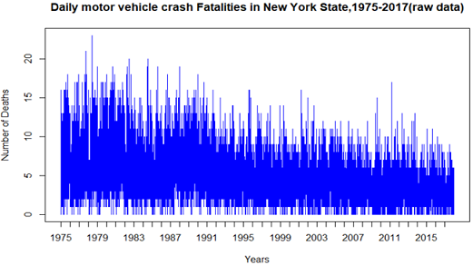
Figure 1.1 Raw data, Time series plot of crash fatalities in New York State,1975-2017
The decomposition of time series is needed because it makes it much more simple and clear in order to analyze its components. It can expressed by the equation: y(t)=L(t) + Se(t) + Sh(t),
where y(t) is the time series data in a logarithmic scale, L(t) is the long-term and trend component, Se(t) is the seasonal term, and Sh(t) is the short term component.
To separate its components, Kolmogorov-Zurbenko (KZ) filter was applied [7, 8]. KZ filter with parameter m and k is defined as :
KZm,k[X(t)]= ∑_(k=-((m-1))/2)^(((m-1))/2)X(t+s) x a_s^m,k, where coefficients a_s^(m,k) = (c_s^(k,m))/m^k , s= (-k(m-1))/2 …….. (k(m-1))/2 are given by the polynomial coefficients obtained from equation ∑_(r=0)^(k(m-1))z^r c_(r-k(m-1)/2)^(k,m) = (1+z+…….+zm-1)k
Trend
Figure 1.2 is the time series plot of log-transformed data. The first component extracted is a long-term trend which is represented by the smoothed line in the red color. It describes the fluctuations of time series defined as being longer than one year. To extract the long-term trend component in this analysis, KZ365,3 filter was applied on natural log-transformed data. Its mathematical form is L(t)= KZ365,3[y(t)], where y(t) is time series data in log scale, m=365 days and k=3 iterations. During the log transformation, some invalid data was created as the log of 0 does not exist. All these values were replaced by 0. As it appears in figure 1.2, the trend is decreasing and this has happened continuously after 1994. Simple regression model was used to calculate the slope of the long-term trend which is approximately is -6 x 10⁻⁵ per day. To make it more meaningful it was multiplied by 365 and 100 and the result is -2.2 % annually, indicating that New York State, each year from 1975 to 2017 has seen, on average, 2.2% fewer motor vehicle crash deaths than the previous year.
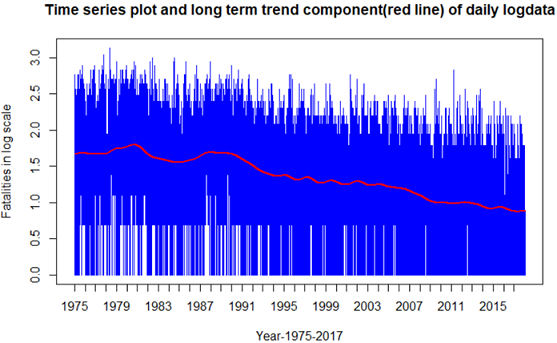
Figure: 1.2 Log transformed data, Time series plot of crash fatalities in New York State,1975-2017. Red line is the long-term and trend which was filtered by using KZ365,3 filter. L(t)= KZ365,3[y(t)]
Seasonality
First, the long-term trend was subtracted from log transform data and the result is seasonality with the short term and error. Seasonality(t)+Short(t)=y(t)-L(t), where y(t) is the time series data in log scale and L(t) represents the long-term trend component. Afterward, KZ29,3 was applied to remove short term and the remainder where m=29 days and k=3 iterations. Mathematically, seasonality can be expressed as Se(t) = KZ29,3[y(t)-L(t)]. Seasonality component Se(t) describes year to year seasonal fluctuations. Figure 1.3 is the seasonality plot after these two operations were applied. As appears in this plot, there is a strong seasonality within one-year period. Summer and winter appear to be the highest and lowest point for each year and this appears to happen approximately every six months. On average, the range of values between peak and off-season each year is approximately 0.5 in log scale or 50% as a percentage reading. In other words, in average, summer has approximately 50% more crash fatalities compared to winter season.
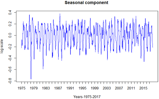
Figure: 1.3 Log transformed data, Seasonality plot of Crash Fatalities in New York State,1975-2017, Seasonality(t) = KZ29,3[y(t)-L(t)].
Driving at night is more of a challenge than many people think. It is also more dangerous because of the darkness. Depth perception, color recognition, and peripheral vision are compromised after sundown. Older drivers have even greater difficulties seeing at night. It is known that most of the motor vehicle traffic flows are in the morning from 6:00 - 9:30 am and afternoon 3:00 - 7:00 pm. In New York State, day light savings time makes a difference in the available light between fall and spring. Because of the day light savings time in the fall, the interval of time 4:00 - 7:00 pm, one of the peak period of motor vehicle traffic, will mostly be in the dark, creating even more dangerous condition.
To assess if this change influences the number of crash fatalities, seasonality component was averaged daily and its plot is displayed in figure 1.4. It is the daily average plot of crash fatalities in a logarithmic scale for all 43 years data. As shown in this figure, it is simple to notice that the end of February and beginning of March are the safest weeks for the drivers to be on road because in these days, approximately, there are 28 % less crash fatalities compared to the average. Late summer appears to be the time period with most of the crash fatalities, approximately 20 % more than average. Dashed line is a cosine wave approximation of daily average crash fatalities and by looking both lines, it is noticeable that after late September, our red line deviates from its previous behavior.
The vertical shadow area in figure 1.4 is approximately the historical time interval of day light savings time in the fall. Even though it is not very clear, this interval corresponds to a reasonable bump in the average line of crash fatalities, that is due to time change in fall.
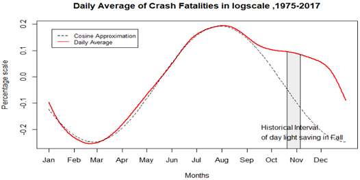
Figure: 1.4 Log transformed data, the daily average plot of Crash Fatalities in New York State,1975-2017 in log scale. Dashed line is cosine wave approximation. Shadow area is the historical interval of day light saving time in Fall.
Short term
Short term component was extracted by using the formula Sh(t)=y(t)-L(t)-Se(t), where Sh(t) -short term information plus error, y(t) is the time series data in a logarithmic scale and Se(t) represents the seasonality component. The short term component contains a weekly scale but also the error term. Its plot is displayed in figure 1.5. As shown, the mean is approximately 0 and this means that the decomposition model was correctly chosen.
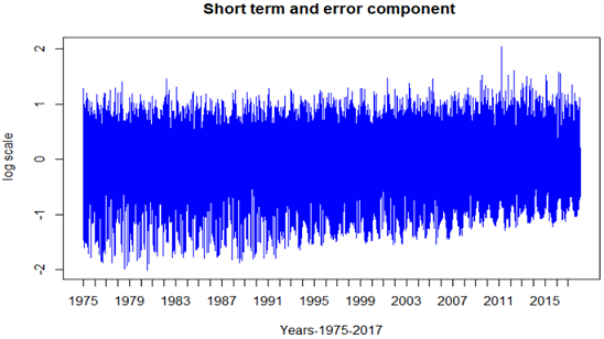
Figure: 1.5 Log transformed data, Weekdays average plot of Crash Fatalities in New York State,1975-2017 in log scale.
The short term component was used to get the weekdays average of motor vehicle crash fatalities. It is displayed in figure 1.6. Saturday has the highest deviation from the average weekdays, approximately 27 % above and Tuesday is 17% below it. According to this plot, Saturday seem to be the worst day to drive because it is the highest point and on average, it has approximately 45 % more crash fatalities than Tuesday which is the lowest point in this graph.
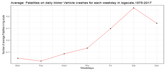
Figure: 1.6 Log transformed data, Seasonality plot of Crash Fatalities in New York State,1975-2017. Sh(t)= y(t)- L(t)-Se(t)
To assess the day light savings time effect in another manner, the weekdays average was calculated from 1975 to 2017 for the days in the interval two weeks after the time changed in each fall season in original scale, which is in blue color in figure 1.7. The red line represents the general weekdays average in original scale and it is almost the same as what was shown in the logarithmic scale in figure 1.6 and the dashed lines around it highlight the 95 % confidence region for the weekdays average number of crash fatalities.
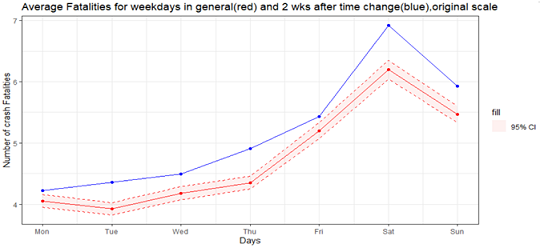
Figure: 1.7 Red line represent weekdays average from 1975 to 2017 and shadow area is 95% confidence region for average number of accidents. Blue line represents weekdays averages only two weeks after day light saving time in fall on the original scale.
In this plot, the day light savings time effect appears to be clear because the blue line is over the red line region for all weekdays. By considering the differences between blue and red line for each weekday, it was calculated, on average, approximately three more crash fatalities occur per week after the day light savings time change in the fall. In total, for 43 years, this number becomes approximately 258 crash fatalities as is shown below:
(2 weeks after day light savings time ) x (approximately 3 fatalities per week on average) x (43 years) ≈ 258 fatalities.
In conclusion, for New York State, the time change in November is shifting evening commute from a brighter time to a darker time and thereby, making evening traffic much more challenging.
Identify sudden change points
Another great operation of Kolmogorov-Zurbenko (KZ) filters family is Kolmogorov -Zurbenko Adaptive (KZA) filter which was developed to detect breaks or change-points in the data[9]. The KZA filter adjusts the size of the head and tail in response to the change in the spline created with KZ. The head of the filter will shrink in response to an increase in slope of the spline and as effect it will zoom in on the change point.
Figure 1.8 is the time series plot in a logarithmic scale and the red line was filtered by using KZA filter. As shown there, the red line has some discontinuous points which were detected by using this filter
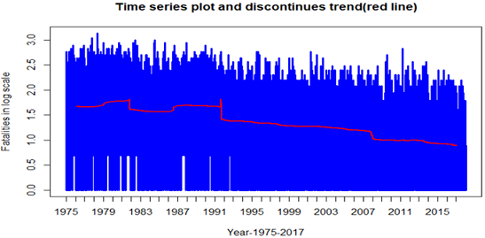
Figure: 1.8 Blue color part is the plot time series in log scale and red line represent the sudden changes of trend at different points of time.
To clarify more on these changes point, the same result of the KZA filter was plotted over only the long-term trend component which is displayed in figure 1.9 These three time points, where most of the level in the trend had changed, were identified as shown in this plot in three different intervals which are in 1981-1983,1990-1992 and 2007-2009. These time intervals are represented by three vertical lines in different colors. According to the National Bureau of Economic Research in the United States, these time intervals correspond to recession periods in these years. When a recession happens, a complex combination of changes impacts the traffic volume on the road. In this kind of situation, the unemployment rate increases and this can decrease miles per person traveled in each day which is directly related to motor crash fatalities.
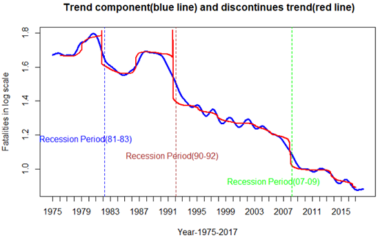
Figure: 1.9 Blue line is the plot of long-term trend in log scale and red line represent the sudden changes at least in three points of the trend. These three points correspond to recession years in the US.
Although, by visually looking these arguments are related to crash fatalities, one question naturally arises: do the national recessions years align with New York State’s Economic recessions and is there any statistical evidence that supports a relation-hypothesis? To answer this question, in figure 1.10 the monthly unemployment rate, which is one of the recession indicators, is plotted against monthly crash fatalities for years between 1976 and 2017 in original scale after the trend component was removed.
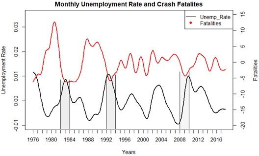
Figure: 1.10 Red line is long-term component of monthly crash fatalities and black line represent unemployment rate long term component. Vertical shadow areas correspond to highest unemployment rate and lowest crash fatalities for New York State.
The shadowed areas correspond to year intervals with the highest rate of unemployment and the lowest numbers of crash fatalities. These are almost the same intervals we discussed in figure 1.9, when U.S Economy had been in a recession. Cross correlation between these two variables is approximately 0.5 and this is a further indicative of a relation between crash fatalities and economic recessions.
Another conclusion from figure 1.9 is that the recession happened in the 90-92 period had the highest impact on crash fatalities behavior which is shown by a brown vertical line. To assess how the level and trend had changed, an interrupted time series or otherwise known as a segmented regression, was used [10]. This model with single outcome requires basically three time periods.By considering recession in 1992 as intervention or another external factor happened, then all years before, from 1975-1991 are defined as pre-intervention and years after, 1993-2017 as post-intervention. Mathematically, this model can be written as below:
Fatalities=b0+b1xTime+b2xIntervention+b3xTime_After+error, where time is a count variable which simple counts days from first to last day included in dataset, intervention is a binary indicator variable defined 0 for pre-intervention period and 1 for the post-intervention time period, and, time_after is a variable that takes 0 for preintervention time and counts each time point after post-intervention. Beta – parameters were estimated by using the Generalized least squares method and it was chosen because of the correlation that is present in our daily data.
In figure 1.11 is the plot of results for this analysis. The shadowed area represents the wash period year which in this scenario is 1992, the year when mostly this recession might have impacted the behavior of crash fatalities in New York State. As shown there, the level of crash fatalities has decreased by approximately 15 % and the trend change is very small with less than 1 %. The counterfactual effect is an imagery line that shows the trend that would have occurred if the recession did not happen.
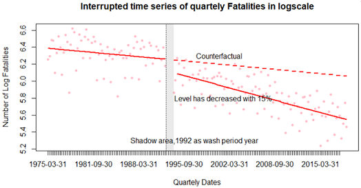
Figure: 1.11 Interrupted time series plot of quarterly Fatalities in log scale. Shadowed area represents 1992 as the wash period year. 90-92 recession had decreased with approximately 15 % the level of crash Fatalities.
Spectral Analysis
One of the most interesting parts of this time series analysis was the spectral analysis because of the surprising frequencies that were hidden in the motor crash fatalities data in New York State. To investigate longer periodicity in crash fatalities, the first KZ730,3 filter was applied on log seasonality and short term Sh(t) and in this way, annual and shorter periodicity were removed. After, the KZP algorithm with parameter m= 15706 days (all days in data), k= 1 iteration and the DiRienzo-Zurbenko (DZ) smoothing parameter=0.002% was applied to investigate if longer periodicities were hidden in the motor crash fatalities in New York State. As appears in figure 1.12, the highest frequency corresponds to 10.7 years periodicity or approximately 11 years and the lower one corresponds to 6.1 years periodicity. Another result in this analysis was a frequency corresponding to one year periodicity. It is excluded from this plot because we identified it in seasonality component analysis and here we were interesting to identify smaller frequencies that correspond to longer than one year periodicity. The 11 years periodicity is a very surprising and interesting result because it is approximately the same with 10.8 period in sunspots which have been studied very well from Professor Zurbenko in his past researches.
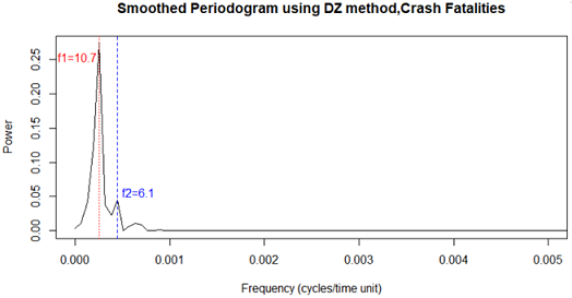
Figure: 1.12 Fatalities spectra from the application of KZP algorithm with parameters m=15706 and k=1 and DiRienzo-Zurbenko (DZ) smoothing parameter .002%. f1 corresponds to 10.7 years and f2 corresponds to 6.1 years.
In figure 1.13, a sunspots periodogram is displayed, which was generated by using KZP(Kolmogorov-Zurbenko Periodogram) algorithm with m=3235 months ,k=1 iteration and DiRienzo - Zurbenko (DZ) smoothing parameter= 8%.[15] Red vertical lines were drawn at the highest spike and its frequency corresponds to 10.8 years period. It is unbelievable that a long period of motor crash fatalities in New York State is almost the same as sunspots which was almost 11 years and 90 years. Professor Zurbenko and his students had shown before in different researches that sunspots activity impacts our life in different areas such as the skin cancer cycles (Edward Valachovic, Igor Zurbenko,2014), seasonal differences in diabetes mortality correspond to seasonal trends in sun activity (Stella Arndorfer, Igor Zurbenko,2017). Also, he has shown in many studies that sunspot activity is strongly associated to the Earth’s climate changes. These changes also might be related to motor vehicle crash fatalities because of the weather conditions. Further analysis would be needed to investigate these hypotheses or to identify other factors that are associated with motor vehicle crash fatalities in New York State
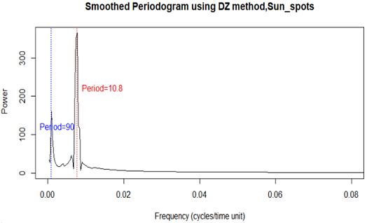
Figure: 1.13 Sunspots spectra from the application of KZP algorithm with parameters m=3235 and k=1 and DiRienzo-Zurbenko(DZ) smoothing parameter 8%. Blue vertical line corresponds to 90 years period and red one corresponds to 10.8 years or approximately an 11 year period.
Result and Discussion
As we saw the first plot, analyzing this time series data would not have been possible without the decomposition process. Using KZ(Kolmogorov-Zurbenko) filter, we successfully decomposed the time series in its main components based on the additive model in the log scale. We then analyzed each component separately and the interesting results we saw for each case. The strongest component was the trend and we found that motor vehicle fatalities are decreasing approximately 2.2% each year. If, in 2017, there were 999 crash fatalities in New York, this means that for 2018 would be on average approximately 22 fewer motor vehicle crash fatalities. In seasonality component analysis, the yearly cycle was clearly present with periodic peaks mostly in each summer. Day light savings time in the fall had an effect in increasing of crash fatalities in two weeks after it changes back one hour compared to average weekdays motor vehicle crash fatalities. Based on data in the original scale, it was calculated on average there were 3 more fatalities in the week after day light saving time and for the course of 43 years, this number becomes approximately 258 additional crash fatalities for all of the two weeks post day light savings time change. Moreover, we saw that on average, Saturday was the day with the highest crash fatalities and Tuesday was the best day to drive because it had the fewest fatalities of all the days of the week.
KZA(Kolmogorov-Zurbenko Adaptive) filter was used for identifying suddenly changes and as we showed above, there were three such time periods which corresponded with economic recessions in the US. Based on cross correlation, it was enough evidence to support the hypothesis that Economic recessions and crash fatalities are statistically correlated. By using Interrupted Time Series, we estimated that the 90-92 Recession period had decreased motor vehicle crash fatalities in New York State with approximately 15%. Spectral analysis provided a very interesting result. One-year periodicity was present and this result was suggested by seeing the plot of seasonality component. An unexpected result, however, is the 10.7 years period which was shown by the spectra plot. The strongest periodicity on the solar cycle is approximately 11 years and this correspondence might be indicative of a solar electromagnetic activity effect on motor vehicle crash fatalities in New York State, an option which may further be explored in the future. Limitations to this analysis include the possible data error and another limitation is that data was only for New York State. This analysis could be improved by using entire US crash fatalities data and having hourly records could be more helpful and make the study more encompassing and accurate.
Conflicts of Interest (COI) Statement
Authors report no conflict or competing interest.
References
World Health Organization.View
NYSDOH.View
National Highway Traffic Safety Administration.View
Fatality Analysis Reporting System.View
Close, B., Zurbenko, I., Sun, M., & Kolmogorov-Zurbenko . (2018). adaptive filters, KZA, version 4.1.0, R-software.View
Zurbenko, Igor., & Sun, Mingzeng. (2017). Applying Kolmogorov-Zurbenko Adaptive R-Software. International Journal of Statistics and Probability. 6. 110. 10.5539/ijsp. v6n5p110.View
Zurbenko, I.G. (1986). The spectral analysis of time series. North-Holland series in Statistics and probability. Elsevier Science, Amsterdam, New York.View
Yang, W., and Zurbenko, I. (2010), Kolmogorov–Zurbenko filters. WIREs Comp Stat, 2: 340-351. doi:10.1002/wics.71View
Zurbenko, I.G., and Smith, D. (2018). Kolmogorov–Zurbenko filters in spatiotemporal analysis. WIREs Comput Stat, 10: e1419. doi:10.1002/wics.1419.View
Use of Interrupted Time Series Analysis in Evaluating Health Care Quality Improvements.View
Time Series Analysis on Diabetes Mortality in the United States, 1999-2015. View
Skin Cancer, Irradiation, and Sunspots: The Solar Cycle Effect, Edward Valachovic, Igor Zurbenko.View
An efficient Prediction Model for Water Discharge in Schoharie Creek, NY. Katerina G. Tsakiri ,Antonios E. Marsellos ,Igor G. Zurbenko.View
Wikipedia Kolmogorov – Zurbenko Fiter.View
DiRienzo, A. G., and Zurbenko, I. G. (1999). “Semi-adaptive nonparametric spectral estimation,” Journal of Computational and Graphical Statistics, vol. 8, no. 1, pp. 41–59.View
Time Series Analysis and Forecast of Crash Fatalities During Six Holidays Period.View
Zurbenko, I. G. & Potrzeba, A. L. (2019). Solar Energy Supply Fluctuations to Earth and Climate Effects, World Science News 120(2):111-131. View
Potrzeba-Macrina, A., & Zurbenko, I. (2019). Periods in Solar Activity, Advances in Astrophysics, Vol. 4, No. 2, May 2019, , Advances in Astrophysics, Vol. 4, No. 2. https://dx.doi. org/10.22606/adap.View
Zurbenko, I. G., & Potrzeba-Macrina, A. L. (2019). Analysis of Regional Global Climate Changes due to Human Influences, World Scientific News, WSN 132:pp 1-15.View
Yang, W., & Zurbenko, I. (2010). Nonstationarity, Wiley Interdisciplinary Revives in Computationa Statistics, Wiley, 2,107-115.
W.Yang, W., Zurbenko, I., & Kolmogorov-Zurbenko, F. (2010). Wiley interdisciplinary revives in computational statistics, Wiley, WIREs in Computational Statistics 2:340-351.View
Arndorfer, S., and Zurbenko, I. (1999-2015). Journal Biom Biostat 2017, 8:6,Time Series Analysis on Diabetes Mortality in the United States, Kolmogorov-Zurbenko Filter DOI: 10.4172/2155-6180.1000384.View
Zurbenko, I., & Sun, M. (2017). Applying KolmogorovZurbenko Adaptive R-Software, International Journal of Statistics and Probability; Vol. 6, No. 5.View
Valachovic, E., & Zurbenko, I. (2017). Separation of SpatioTemporal Frequencies, Quest Journals, Journal of Research in Applied Mathematics. 3:29-37. View
Valachovic, E. & Zurbenko, I. (2017). Multivariate Analysis of Spatial-Temporal Scales in Melanoma Prevalence, Cancer Causes Control, Springer, 2017. doi:10.1007/s10552-017- 0895-xView
Zurbenko, I. and Luo, M. (2015) Surface Humidity Changes in Different Temporal Scales. American Journal of Climate Change, 4,226-238. doi: 10.4236/ajcc.2015.43018.View
Zurbenko, I., & Sun, M. (2017). Applying KolmogorovZurbenko Adaptive R-Software, International Journal of Statistics and Probability; Vol. 6,No. 5.View
Zurbenko, I., & Potrzeba, A. (2009). Tidal Waves in Atmosphere and Their Effects, Acta Geophysica, 58,356-373. DOI:10.2478/ s11600-009-0049-y.View
Close, B., & Zurbenko, I. (2008). Time Series Analysis of the Fatal Accident Reporting System, Proceedings of Annual ASA conference.
Zurbenko, I.G., Cyr, D.D. (2011) Climate fluctuations in time and space, Climate Research, 46,67-76. View
Zurbenko, I., & Potrzeba, A. (2013). Periods of excess energy in extreme weather events, Journal of Climatology, http://dx.doi. org/10.1155/2013/410898View