
- About the Journal
- Editorial Board
- Review Process
- Author Guidelines
- Article Processing Charges
- Special Issues
- Indexing
- Current Issue
- Past Issue
 Journal of Public Health Issues and Practices
Journal of Public Health Issues and Practices Volume 5 (2021), Article ID: JPHIP-174
https://doi.org/10.33790/jphip1100174Review Article
Trajectories Matching for Characterizing Patient’s Behavior in Policy Evaluation
Chaohsin Lin, PhD1,Shuofen Hsu, PhD1,Yu-Hua Yan, PhD2,3*
1Department of Risk Management and Insurance, National Kaohsiung University of Science and Technology, Kaohsiung, Taiwan.
2Department of Medical Research, Tainan Municipal Hospital (Managed by Show Chwan Medical Care Corporation), Taiwan.
3Department of Hospital and Health Care Administration, Chia Nan University of Pharmacy and Science, Taiwan.
Corresponding Author Details: Yu-Hua Yan, PhD, Department of Medical Research, Tainan Municipal Hospital (Managed by Show Chwan Medical Care Corporation); Department of Hospital and Health Care Administration, Chia Nan University of Pharmacy and Science, Taiwan. E-mail: 2d0003@mail.tmh.org.tw
Received date: 07th December, 2020
Accepted date: 08th January, 2020
Published date: 13th January, 2020
Citation: Lin, C., Hsu, S., & Yan Y.H. (2021) Trajectories Matching for Characterizing Patient’s Behavior in Policy Evaluation. J Pub Health Issue Pract 5(1): 174.
Copyright: ©2020, This is an open-access article distributed under the terms of the Creative Commons Attribution License 4.0, which permits unrestricted use, distribution, and reproduction in any medium, provided the original author and source are credited.Creative Commons Attribution License, which permits unrestricted use, distribution, and reproduction in any medium, provided the original author and source are credited
Abstract
Background: Economic theory and earlier empirical evidence suggest that patients will use fewer health services when they have to pay more for them. However, that copayment had little or no effect on visits to physicians.
Objectives: This study exploits a natural experiment in Taiwan to estimate the effect of an increase in copayment on the demand for physician services and prescription drugs across the different dimensions of age, illness severity and patient behavior.
Methods: Data were taken from the National Health Research Institute (NHRI) in Taiwan for the period of 1998 to 2000 and contained enrollment and claims files from a randomly chosen 0.2% of Taiwan’s population. The deletion of observations with missing values for any of the dependent or independent variables resulted in a final sample size of 69 768 individuals. The basic empirical strategy is to pool the data over the two years in question and estimate the effects of the reform by comparing the expected number of visits before and after the reform. We explored several alternatives stratifying the treatment in order to improve the quality of the identification.
Results: We found that the reduction in visits was rather conservative with the DD estimates ranging from -0.08 to -0.17 compared to the estimate of -0.38 without stratification. The reform effect will most likely be exaggerated if the unobserved heterogeneity of the individual, such as health status and behavior, is not considered in the model.
Keywords: Trajectories, Patient’s Visiting Behavior, Copayments, Morbidity Risk
Introduction
This study constructed two trajectories of patient’s medical cost incurred and his/her predicted morbidity respectivelyin assessing the effect of health policy. It is well known that randomly assigning a control group is important in the assessment of policy reforms or new interventions [1]. However, it may not always be possible for researchers to implement a randomized experiment. Therefore, most literature relied on a natural experiment under a National Health Insurance (NHI) scheme where certain groups of the population exempted from the cost sharing mechanisms are natural candidates for the control group [2]. The difference of the change in medical utilization before and after the reform between the treatment and control group, i.e.,the difference-in-difference (DD) estimation, was a measure for evaluating the impact of thepolicy reform.
However, under an NHI system the exemptions were most often granted to recipients of certain government benefits such asthose for income support or disability. There is an endogeneity problem when the division into treatment and control is based on welfare and low income. In addition, a shortcoming of the natural experiment is the lack of controls for unobserved person specific heterogeneity. Thus, the candidates for the control group may be too different to provide good matches for those in the treatment group [3]. This type of heterogeneity is important in assessing the reform effect for two reasons. First, an unobserved individual’s health risk may generate significant influences on health care demand, which should not be attributed to the price effect of the increases in cost sharing. Second, behavioral idiosyncrasies such as the propensity to seek health care given the same morbidity level might differ in unobservable but systematic ways between individuals. Therefore, it is not surprising that the empirical results regarding the cost containment effect onthe demand sideof healthcare is mixed in the literature [4,5] and left open to address. An approach which allows one to control for the unobserv ables improves the quality of the comparison group and the efficiency in assessing policy effect. In this study we proposed an index to characterize an individual’s behavior of seeking healthcare. Using Taiwan’s NHI data as an illustration, we demonstrate how to evaluate the reform effect across heterogeneous patient’s visiting behavior.
The remainder of this paper is organized as follows. In the next section, we first show how to construct an indicator for characterizing the patient’s visiting behavior. In particular, two trajectories of the patient’s morbidity and healthcare utilization are devised respectively for this purpose. We then provide a brief description of the copayment reform under Taiwan’s NHI and the data that was employed in this study. The empirical results in the different models w/ and w/o incorporating the index for patient’s visiting behavior are presented in Section 3 while Section 4 discusses the reform effects w/ and w/o the stratification of patient’s visiting behavior. We draw our conclusions in section 5.
Methods
For each individual, we constructed two trajectories: one using predicted resource indexand the other using the number of doctor visits actually incurred. On the one hand, a trajectory for the number of outpatient visits an individual incurred, i.e., doctor visittra jectory, was constructed using two observations: one based on data from the pre-reform period while another from the post-reform period. On the other hand, the Johns Hopkins Adjusted Clinical Group (ACG) [6] Case-mix System was employed to predict an ACG morbidity measure for each patient as the benchmark index reflecting his/her health risk.
An individual’s health risk was usually measured through the information from survey, laboratory or claims data. Survey or laboratory information could not be obtained on a large scale given the cost consideration, while claims data is easily accessible in a healthcare system requiring electronic claims submission for reimbursement, such as in Taiwan. The Johns Hopkins ACG Casemix System is one of the most popular risk adjustment systems that can be used to evaluate an individual’s health risk using claim data7. Even though the ACG system was developed in the United States, it has been adopted globally, including many European countries, Canada and some Asian countries [7-15]. Research has shown that the performance of the ACG system in Taiwan is comparable to that of the United States [10,16]. The ACG morbidity measures are a series of mutually exclusive, health status categories defined by morbidity, age, and sex and are used to determine the morbidity profile of patient populations to allow for more equitable comparisons of utilization across two or more patients. A higher predicted ACG index indicates that the individual has a greater morbidity burden as well as a higher health risk and is assumed to consume more than the average amount of health services in the future. The variation trend of the patient’s ACG indexes over successive periods can be thought of as that patient’s “morbidity trajectory” or “health risk trajectory” [17]. Improvements or deteriorations in a person’s predicted health status can be found through the variation trend of his/her health risk trajectory, which could explain a large portion of the reduction/ increase in the number of doctor visits. Thus we should control for that changes in health status in order to assess the price effect of the reform.
From the pre to post period, three possible patterns of change for each of the above two trajectories could be identified: increasing, decreasing, or erratic. By contrasting the two trajectories with three patterns each, nine combinations were possible. For patients with the two trajectories of the same pattern (both increasing, both decreasing, and both erratic), we assume that doctor visits are mostly attributed to individual’s morbidity burden because the variation of the two trajectories coincide with each other. Under such circumstances, the changes in medical utilization should not be attributed to the policy reform because its variations reflect the results of a patient’s health risk, i.e., their true medical needs. On the other hand, individuals in the remaining combinations are of two kinds. One is featured by the overconsumption of medical resources when morbidity trajectory is decreasing whilst the doctor visits trajectory is increasing or erratic ,or where morbidity trajectory is erratic but the doctor visits trajectory is increasing. Individuals with one of these patterns are likely to incur moral hazard because the variations in their actual medical utilization are constantly higher than those in their predicted morbidity level. We defined individuals with these patterns as MH group. The other is constituted by the rest in which individual’s actual medical utilization is less than her/his morbidity burden.
Data source and study subjects
As an illustration of the proposed methodology, this study employed Taiwan’s NHI claims data prepared by the National Health Research Institute (NHRI) between January 1, 1998 and December 31, 2000, within which a major policy change in copay ment occurred. Ever since the implementation of the compulsory single-payer program, Taiwan’s NHI adopted various measures to constrain the rapid increase in outpatient costs. There were several amendments to the copayment system. However, the reform initiated in 1999 was the biggest given the large and multifaceted impact on the health coverage of the people in Taiwan. Beginning on August 1, 1999 the NHI implemented a new copayment system which substantially increased the copayment rate to 20% for ambulatory care and outpatient prescription drugs for all but two insured categories: (1) those insured with a low-income status as qualified by the Social Support Law, and (2) veterans and their survivors. The fact that people belonging to these two insured categories are left unaffected by the new copayment system allowed us to construct a natural control group for performing DD estimation in evaluating the reform effect.
The data contained enrollment and claims files from a randomly chosen 0.2% of Taiwan’s population (approximately 20 million individuals). The enrollment files contained individual subscription information and demographic factors, including sex, date of birth, and the category of the beneficiary based mainly on occupation and income. The claims files contained comprehensive records of utilization of ambulatory care including date of service, the International Classification of Diseases, Ninth Revision, Clinical Modification (ICD-9-CM) diagnosis codes, claimed medical expenses, and the amount of copayment for each encounter. We dropped the observations in the year 1999 (when the policy reform occurred) to avoid transition effects3. We included subjects with at least one calendar year of enrollment before (1998) and after the reform (2000) and without missing values on dependent or independent variables. The final sample size was 69,768 individuals.
Empirical model
We built three negative binomial (NB) models to evaluate the impact of the policy reform in copayment on the number of doctor visits. The first model served as a benchmark and included independent variables as follows: 1) a group indicator (treatment group vs. control group); 2) a period indicator (pre- vs. post-reform); 3) an interaction term of group and period; 4) an individual’s characteristics including gender, age, the identity status for major illness ( ). In the second model, we in corporate the constructed index for characterizing the patient’s behavior of doctor visits, i.e., the moral hazard index (MH) in the regression. The variable of interest in the bench mark and the second model is the coefficient associated with the interaction term. If it is negative, the demand for doctor visits in the treatment group falls relative to that in the control group after the policy reform. However, the effect of reform might be expected to vary depending on different patient behavior. Since multiple interactions can be used to define exactly who is exposed to treatment and also to allow for heterogeneity in the size of the treatment effect1. We employed the differences-in-differences-in-differences (DDD) approach to allow for the interaction among the reform, the treatment and the MH which indicated patient’s behavior with moral hazard. In addition to the variables in the second model, the third model thus also included: 1) an interaction terms of MH and the control group indicator; 2) an interaction terms of MH and period indicator; and 3) an interaction terms of MH, control group and period indicator. The last interaction term captures the variation in visits specific to the treatment group (relative to the control group) with specific patient’s behavior of MH (relative to non-MH) after the reform (relative to before the reform), and is therefore the DDD estimator of the reform effects on doctor visits.
Results
Descriptive statistics
As shown in Table 1, the sample ratio of treatment and control group is 86.5% vs. 13.5%, respectively. The average number of visits decreased significantly (t=-5.19) after the reform for the treatment group, but did not change significantly (t=0.1649) for the control group. This may be due to the fact that the control group has a larger proportion of major illness identity status and of the elderly, which coincides with the expectation from which the demand for medical care is known to increase significantly with illness severity and with age. However, the control group has a smaller average number of visits relative to the treatment group both before and after the reform. This could be due to a difference in other unobservable characteristics associated with patient’s behavior, and subsequent analysis will attempt to address this issue.

Table. 1 Descriptive Statistics
Over all, the composition structures of age, gender,major illness identity statusand MH differed significantly across the two groups both before and after the reform. The χ2 tests for independence rejected the null hypotheses at the 0.05 significance level. In addition, the two-sample test with unequal variances also rejected the hypothesis that the mean values of these control variables were equal. In specific, the female ratio of the control group is lower than that of the treatment group. The higher average age of the control group was mostly due to a higher proportion of individuals aged 65 and above.
The MH sample ratio in the control and treatment group is almost equivalent (21.1% vs. 21.9% respectively). The visits of MH group after the reform are not only larger than those of non-MH group but also larger than the total average visits. The discrepancies of visits between MH and non-MH for the control group after the reform are almost 2 times those for the treatment group. It indicates that the effects of the reform may be an illusion if the heterogeneous visiting behavior between treatment and control group is not well controlled for. It also explains, although in part, the above mentioned phenomenon of the slightly increased visits in the control group after the reform.
Results in the different models
Two sets of the regression w/ and w/o incorporating the MH variable respectivelyare performed using a variety of the pooled NBs and the panel NBs. The results are displayed in Table 2. In the pooled NBs the standard errors were adjusted to account for the heteroscedasticity of the unknown form and the correlation between observations for the same person. The parameters of the fixed-effects negative binomial (FENB) model were estimated using the conditional maximum likelihood function [18]. In it the mean is homogeneous without shifting the conditional mean function by the fixed effect, so that both the overall constant and the time invariant covariates are allowed in the model.

Table 2. Reform Effects in Different Models
The results were similar across differentestimation techniques. Models that included the dummy variable MH, which indicatesthat an individual’s variation in doctor visit trajectory out-raced that of his/her health risk trajectory of ACG morbidity burden, offered a substantial improvement as reflected both infavorableSchwartz Information Criterion (SIC) and the Akaike information criterion (AIC). The effect of the reform indicated by the interaction term of policy reform and the treatment group was negative with statistical significance in all cases. Women andthe elderly had more visits,which agreed with the literature. Both coefficients of the MH and the treatment group were all significantly positive.
However, the estimated parameters differed slightly between the two specifications of the pooled and the panel NBs. First, the coefficient of the reform dummy indicated that there was a statistically significant increase in the expected number of visits after the reform for the panel model, while it wasnegative although statistically insignificant otherwise.The increase associated with reform itself is not converted to the expected decrease due to the interaction effect of treatment and reform. Besides, the increase in the year dummy may also arise from the rising income, the new technology in medicine, improvements in access to clinical services and better quality of healthcare that resulted in a yearly increase in outpatient utilization. Second, individuals with a major illness identity (MI-ID) had more visits for the pooled but less visits for the panel estimation. A possible explanation for this may beowing to the factthat individuals with a MI-ID can receive free refills from pharmacies other than from clinics following their initial doctor visit.
The above ambiguity between these estimated coefficients may be attributed to the distinct nature among different model specifications. It should be noted that the longitudinal data employed in the current study is a rather short panel with only two periods of observations for a given person. The presence of an individual specific heterogeneity term would invalidate the assumption of independent sampling. Since FENB accounts for the latent heterogeneity and for its correlatedness with the exogenous variables [1,19], it follows that the estimation results from FENB are much more robust and efficient than those from the other alternatives. Both the SIC and the AIC suggest a preference for the FENB specification. In addition, the Hausman test also rejected the random specification and confirmed the evaluation that the FENB corresponds to the data.Thus, we focused on FENB in the following DD and DDD estimations.
Discussion
Reform effects
The bootstrapping results of the DD estimates are shown in Table 3, which is computed as follows.
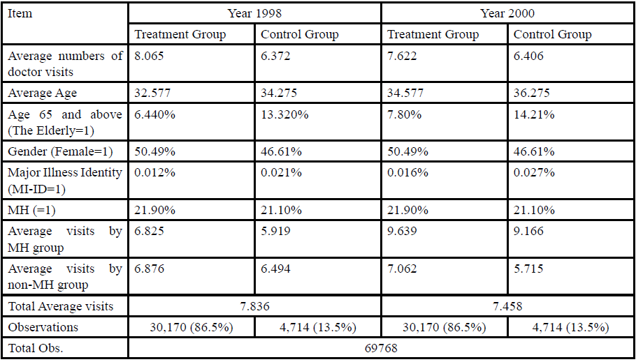
Table. 3 DD Estimates
Where yitˆit y is the estimation for the number of doctor visits, g=1, 0 denotes for thetreatment and the control group, t=1. 0 denotes for the pre- and postreform, SDg=1 and SDg=0 are simple difference (SD) in the pre-post change of the estimated numbers of doctor visits for the treatment and control group, respectively.The reform effect (DD) is negative in all cases and is statistically significant as shown in Table 3. Compared to the other NB specifications, the FENB generates the most conservative estimate of the reform effect, amounting to a reduction of -0.15 and -0.39 in the expected number of visits for the treatment group relative to the control group, w/ and w/othe variable of MH included among the regressors respectively. It is obvious that the reform effect is left almost half when the heterogeneity in patient’s visiting behavior of the MH variable is controlled.
The DD estimator can be further decomposed intotwo components of SDg-1 and SDg-0 based on the above Eq. (1). With the MH variable included among the regressors, i.e., Model 2 in Table 3, and again based on the FENB model, the expected number of visits for the control group increased by 0.97. The expected number of visits for the treatment group also increased by 0.83, It is obvious that the increase of the doctor visits in the control group after the reform is larger than that in the treatment group thus resulting in the overall reform effect of a 0.15 reduction. Since the exemptions for copayments in an NHI scheme are most often deliberately granted to vulnerable citizens, it is possible that the patient’s visiting behavior exhibited substantial differences between the treatment and control group. We employed the DDD regression using the constructed MH index to see if this is true.
Reform effects across different patient’s behavior
The results of the DDD regression are shown in the last column of Table 2. It can be noticed that for treatment group with MH behavior, the presence of co-payment leads to a small but insignificant decrease (-0.010) in doctor visits. Moreover, the coefficient of the reform effect turns positive (0.783) with statistical significance. The reform appears to have no constrained effect when certain patients’ moral hazard behaviors are controlled in the model.To further investigate whythe reform appears to have no constrained effect from the above DDD approach and to examine how patients with moral hazard behavior respond to copayment reform differently between treatment and control group, we calculated the within-group DD controlled for patient’s behavior as follows:
Using Eq. (2), the DDD estimator can be decomposed into effects that are induced by moral hazard and that are the change in genuine health needs.In specific, each bracket in Eq. (2) constituted a SD of the pre-post comparison within the treatment and control group respectively under certain patient’s behavior. The bootstrapping results of the above DDD estimation are shown in Table 4 where each cell contains the mean of SD in the average number of visits along with the standard errors and confidence intervals. The first two brackets of SDsin Eq. (2) compare changes in doctor visits for MH group. They not only showed the variations in medical utilization over time, but also the MH individual’s behavioral response to the policy reform. On the other hand, the last two brackets of SDsin Eq. (2) indicate the changes in medical utilization over time for non- MH group and reflect the individual’s genuine needs for healthcare. Subtracting the above two sets of SDs respectively for patients with behavior of MH and non-MH yields two DD estimatorsas shown in Table 4. It is apparent that the DD estimator is significantly negative (-0.2799)only when individuals belong to non-MH group. On the contrary, when individuals are inclined to have moral hazard behavior, i.e., MH group, the DD estimator is positive with statistical significance (4.5037). This indicates that for patients whose propensity to consume out-performs their genuine needs for medical care, there is an increase in visits in the treatment group relative to the control group after the reform. Since the treatment group has higher income than do the control group, our result is consistent with the findings that in most countries higher income people actually visited their physician more often than before the co-payments were imposed [20-22]. The difference between these two DDs yields the predicted DDD of 4.7835, which shows a statistically significant increase in doctor visits. Thus, the reform appears to have no constrained effect when patient’s moral hazard behavior is incorporated in the model.

Table 4. DDD Estimate
The DDD approach thus constructed can alleviate the possible selection bias caused by the unobserved individual’s heterogeneous behavior as follows. The individual’s health risk is generally time varying and unobservable, and thus cannot be subtracted or eliminated by the DD approach. The ACG predicts an individual’s morbidity burden and served as a benchmark for indicating an individual’s health risk. The discrepancies over time between the ACG estimates and real consumption of medical resources can thus be attributed to those causes that are other than patient’s genuine needs for health care. The selection bias caused by the time varying unobserved behavioral factor, i.e., the individual’s moral hazard, can thus be well controlled for. Although there is evidence suggesting the validity of incorporating morbidity factors for improving prediction in future medical utilization and health outcomes [8,13,15,23], to the best of our knowledge, there is not yet an application of the ACG system with the aim of identifying patient’s visiting behavior for improving the assessment of the reform effect.
Implications for Behavioral Health
In this study we constructed an index indicating whether an individual is vulnerable to the behavior of moral hazard by matching two trajectories of the ACG morbidity estimate with actual medical utilization. We demonstrated the validity of the proposed methodology with an illustration of how to identify the differences in outcomes caused by the individual’s heterogeneous behavior in assessing the policy effects. The effect is found to be less profound when the heterogeneity in patient’s visiting behavior is controlled. We showed that the estimated reform effect would be an illusion and be misleading if the patient’s visiting behavior is not incorporated in the model. The proposed methodology can be equally applied to the evaluation of other health policy reforms and/or interventions in which patient’s behavior plays an important role in the outcomes of health and medical utilization.
Conflict of Interest Statement:
The authors declare no conflict of interest.
Declaration of Competing Interest: None declared.
Availability of data and materials: The datasets used and analyzed are available from the corresponding author upon request.Acknowledgements: None declared
Funding: None declared
Abbreviation: National Health Insurance (NHI); differencein- difference (DD); Adjusted Clinical Group (ACG); fixed-effects negative binomial (FENB); differences-in-differences-in-differences (DDD) ; moral hazard index (MH)
References
Jones, A. M. (2009). Panel data methods and applications to health economics. In: TC Mills, K. Patterson (Eds). Palgrave Handbook of Econometrics. London: Palgrave Macmillan.
Manning, W. G., Newhouse, J. P., Duan, N., Keeler, E. B., & Leibowitz, A. (1987). Health insurance and the demand for medical care: evidence from a randomized experiment. The American economic review, 251-277.View
Winkelmann, R. (2004). Co-payments for prescription drugs and the demand for doctor visits–Evidence from a natural experiment. Health economics, 13(11), 1081-1089.View
Kiil, A., & Houlberg, K. (2014). How does copayment for health care services affect demand, health and redistribution? A systematic review of the empirical evidence from 1990 to 2011. The European Journal of Health Economics, 15(8), 813-828.View
Mortensen, K. (2010). Copayments did not reduce Medicaid enrollees’ non-emergency use of emergency departments. Health affairs, 29(9), 1643-1650.View
Johns Hopkins University Bloomberg School of Public Health (2010). The Johns Hopkins ACG Case-Mix System: Documentation and Application Manual for PC (DOS/WIN/ NT) and Unix Version 9.0. Baltimore, MD: Johns Hopkins University.
Weiner, J. P., Tucker, A. M., Collins, A. M., Fakhraei, H., Lieberman, R., Abrams, C., ... & Folkemer, J. G. (1998). The development of a risk-adjusted capitation payment system: the Maryland Medicaid model. The Journal of ambulatory care management, 21(4), 29-52.View
Carlin, C. S., Feldman, R., & Dowd, B. (2017). The impact of provider consolidation on physician prices. Health economics, 26(12), 1789-1806.View
Buja, A., Rivera, M., Soattin, M., Corti, M. C., Avossa, F., Schievano, E., ... & Ebell, M. H. (2019). Impactibility Model for Population Health Management in High-Cost Elderly Heart Failure Patients: A Capture Method Using the ACG System. Population health management, 22(6), 495-502.View
Chang, H. Y., Lee, W. C., & Weiner, J. P. (2010). Comparison of alternative risk adjustment measures for predictive modeling: high risk patient case finding using Taiwan's National Health Insurance claims. BMC health services research, 10(1), 343.View
Caberlotto, R., Buja, A., Pinato, C., Mafrici, S., Bolzonella, U., Baldovin, T., ... & Baldo, V. (2020). Healthcare services use and costs for a cohort of high needs elderly diabetic patients. European Journal of Public Health, 30(Supplement_5), ckaa166-1101.View
Reid, R. J., Roos, N. P., MacWilliam, L., Frohlich, N., & Black, C. (2002). Assessing population health care need using a claims-based ACG morbidity measure: a validation analysis in the Province of Manitoba. Health services research, 37(5), 1345-1364.View
Rudoler, D., Deber, R., Barnsley, J., Glazier, R. H., Dass, A. R., & Laporte, A. (2015). Paying for primary care: the factors associated with physician self-selection into payment models. Health Economics, 24(9), 1229-1242.View
Shen, Y., & Ellis, R. P. (2002). How profitable is risk selection? A comparison of four risk adjustment models. Health economics, 11(2), 165-174.View
Somé, N. H., Devlin, R. A., Mehta, N., Zaric, G., Li, L., Shariff, S., ... & Sarma, S. (2019). Production of physician services under fee-for-service and blended fee-for-service: Evidence from Ontario, Canada. Health economics, 28(12), 1418-1434.View
Lin, C. & Hsu, S. (2014). Constructing "Behavioral" Comparison Groups: A Difference-in-Difference Analysis of the Effect of Co-Payment Based on the Patient's Price Elasticity. Evaluation & the Health Professions, 37(4), 434-456.View
Chang, H. Y. (2014). The impact of morbidity trajectories on identifying high-cost cases: using Taiwan's National Health Insurance as an example. Journal of Public Health, 36(2), 300- 307.View
Haussman, J., Hall, B., & Griliches, Z. (1984). Economic models for count data with an application to the patents-R&D relathionship. Econometrica, 52, 909-938.View
Greene, W. H. (2008). The econometric approach to efficiency analysis. The measurement of productive efficiency and productivity growth, 1(1), 92-250.View
Cockx, B., & Brasseur, C. (2003). The demand for physician services: Evidence from a natural experiment. Journal of Health Economics, 22(6), 881-913.View
Duarte, F. (2012). Price elasticity of expenditure across health care services. Journal of health economics, 31(6), 824-841.View
Rosen, B., Brammli-Greenberg, S., Gross, R., & Feldman, R. (2011). When co-payments for physician visits can affect supply as well as demand: findings from a natural experiment in Israel's national health insurance system. The International journal of health planning and management, 26(2), e68-e84.View
Danagoulian, S. (2018). Policy of prevention: Medical utilization under a wellness plan. Health economics, 27(11), 1843-1858.View