
- About the Journal
- Editorial Board
- Review Process
- Author Guidelines
- Article Processing Charges
- Special Issues
- Indexing
- Current Issue
- Past Issue
 Journal of Public Health Issues and Practices
Journal of Public Health Issues and Practices Volume 10 (2026), Article ID: JPHIP-253
https://doi.org/10.33790/jphip1100253Research Article
Stochastic Modeling of Epidemic Extinction Under Non-pharmaceutical Public-health Policy Interventions
Lixia Wang*, and Donald Porchia
Department of Biostatistics, University of Florida, Gainesville, FL 32610, United States.
Corresponding Author Details: Lixia Wang, Clinical Assistant Professor, Department of Biostatistics, University of Florida, Gainesville, FL 32610, United States.
Received date: 03rd November, 2025
Accepted date: 20th February, 2026
Published date: 24th February, 2026
Citation: Wang, L., & Porchia, D., (2026). Stochastic Modeling of Epidemic Extinction Under Non-pharmaceutical Public-health Policy Interventions. J Pub Health Issue Pract 10(1): 253.
Copyright: ©2026, This is an open-access article distributed under the terms of the Creative Commons Attribution License, which permits unrestricted use, distribution, and reproduction in any medium, provided the original author and source are credited.
Abstract
Public health interventions can change epidemic trajectories and, critically, can also increase the chance that an outbreak dies out early. We developed a quantitative framework to estimate the probability of epidemic extinction under different strengths of non-pharmaceutical interventions implemented in two subpopulations (low-risk and high-risk). The approach extends a standard compartmental model by incorporating random transmission events and evaluating disease extinction probabilities under alternative intervention scenarios.
We applied the framework to COVID-19 incidence data from Brazil (Johns Hopkins University). Under fitted baseline parameters, the basic reproduction number was approximately R0 = 1.4, indicating that deterministic models would predict sustained epidemic growth. Despite R0> 1, the stochastic framework yields substantial extinction probabilities that can be increased through timely interventions. When the outbreak was seeded by one infectious individual in the high-risk group, the estimated extinction probability under baseline intervention levels was 67.22%. A 40% proportional increase in low-risk interventions (holding high-risk interventions at baseline) increased extinction to 74.93%, whereas the same proportional increase applied only to high-risk interventions increased extinction modestly to 68.43%. Increasing interventions in both groups by 40% yielded a similar extinction probability (75.13%), highlighting that broad population-level measures can achieve near-maximal gains relative to dual targeting at the same scale.
Overall, these results indicate that early, population-wide non-pharmaceutical interventions, particularly those improving compliance or reducing transmission in the larger low-risk group, can meaningfully increase the likelihood of epidemic control even when R0 > 1.
Key words: Epidemic Extinction; Non-pharmaceutical Interventions; Compartmental Model; Markov Chain; Branching Process; COVID-19
Introduction
Public health interventions alter key epidemiological parameters, such as contact structure, transmission rate, and recovery rate, and thereby influence the likelihood that an epidemic will naturally die out. Understanding the mechanisms that govern the probability of disease extinction is fundamental for assessing the effectiveness of non-pharmaceutical interventions. Although deterministic compartmental models have been widely used to study epidemic dynamics, the transmission of infectious diseases is inherently stochastic due to random contact patterns, demographic variability, and unobserved environmental effects. Incorporating stochasticity is therefore essential for capturing the range of possible epidemic outcomes, particularly the probability of stochastic extinction.
In this study, we extend the deterministic compartmental model previously described by Asempapa, R. et al [1] by developing a continuous-time Markov chain (CTMC) representation of the epidemic process and approximating it using a multitype branching process. This hybrid stochastic-deterministic framework enables us to derive the analytical characterization of the extinction probability as a function of intervention strengths. Using COVID-19 incidence data from Brazil (Johns Hopkins University), we conduct numerical simulations to illustrate stochastic trajectories of disease dynamics in different compartments. Extinction probabilities are estimated through simulation of the CTMC and computed directly from the branching-process formulation, providing a comprehensive assessment of how early-stage public health interventions shape the likelihood of epidemic extinction.
This study’s objective was to quantify the probability that an emerging epidemic goes extinct under alternative public-health intervention strategies, with particular emphasis on differential targeting of low-risk and high-risk subpopulations. Extinction probability is a policy-relevant endpoint because it complements the basic reproduction number R0 by translating transmission conditions into the practical likelihood that an outbreak will die out early, thereby informing when broad non-pharmaceutical measures are warranted and how aggressively they should be implemented. Using Brazil-parameterized COVID-19 dynamics, we show that proportional strengthening of interventions in the larger low-risk group produces substantially larger gains in extinction probability than the same proportional increases confined to the high-risk group, and can achieve extinction probabilities comparable to strengthening interventions in both groups simultaneously.
Methods
Deterministic compartmental model
A compartmental model is a mathematical framework in which the population is divided into distinct epidemiological classes (compartments), with individuals in each class assumed to be homogeneous. Such models are typically represented as graphs linking the classes through transfer rates, which in turn define a system of differentia [1] equations governing disease dynamics [2]. Compartmental modeling dates back to W. H. Hamer [3] and has been developed extensively over more than a century. It is interesting to note that the foundations of this entire approach in modern epidemic modeling were created not by mathematicians but by public-health physicians, most prominently Hamer, Ross, Hamer, McKendrick, and Kermack, between 1900 and 1935 [4].
Asempapa et al. [1] proposed an eight- compartment model that stratifies the population into two subgroups: low-risk (including children and adults without underlying conditions) and high-risk (primarily elderly individuals or those with comorbidities). Within each subgroup, individuals progress through susceptible (S), exposed (E), and infectious (I) classes. Infectious individuals may subsequently transition to hospitalized (H), or recovered (R) states, yielding a total of eight epidemiological compartments. The model assumes a large, constant population size N, homogeneity within each compartment, infection rates proportional to the effective contact rate, and constant parameter values.
For clarity and ease of reference, we briefly summarize the structure of this model and the key results relevant to our analysis. After incorporating an underlying deceased (D) compartment, the resulting flowchart of the extended model is illustrated in Figure 1.
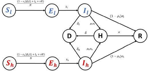
Figure 1
Figure 1. Deterministic compartmental model with low-risk and high-risk subpopulations. Flow diagram of the extended compartmental model stratified by risk group (low-risk: S1, E1, I1; high-risk: Sh, Eh, Ih) with shared hospitalized (H), recovered (R), and deceased (D) compartments. Arrows denote allowed transitions and model flows; parameters governing each transition are defined in Table 1.
Here, Sl, El, and Il represent the Susceptible, Exposed, and Infectious groups, as well as their corresponding population sizes within the low-risk population, respectively. Similarly, Sh, Eh, and Ih denote Susceptible, Exposed, and Infectious groups and their associated population sizes in the high-risk subpopulation, respectively. The compartments D, H, and R refer to the Deceased, Hospitalized, and Recovered groups and their population sizes, respectively. The population sizes of all nine compartments vary over time.
The corresponding deterministic compartmental model is then described by the following system of differential equations, with parameter definitions summarized in Table 1:
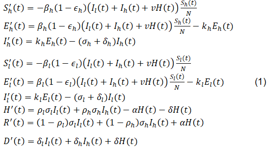
equation1
The basic Reproduction Number R0, which is the average number of infectious individuals generated by one infected individual introduced into the entire susceptible population over the entire duration of the infectious period, is given by

equation 2
Here, Sl(0) and Sh(0) denote the initial sizes of the susceptible populations in the low-risk and high-risk subgroups, respectively, and Sl (0) + Sh (0) = N.
Table 1. Model parameters and definitions for the deterministic compartmental model. Definitions of parameters used in system (1) and Eq. (2), including transmission/contact rates, intervention parameters ε1 and εh, progression rates, hospitalization/recovery rates, and mortality rates. Units are day⁻¹ unless otherwise specified; dimensionless parameters (e.g., proportions) are indicated.
As noted in Asempapa, R. et al [1], for COVID-19, values of certain parameters in the model, such as kl,kh,σl,ρl, can be obtained from related epidemiological studies, while others, including βl,βh,ϵl,ϵh, can be estimated by fitting the model to available data. Specifically, the default parameter values referenced from previous studies are summarized in Table 2 (units for all parameters in Table 2 are day-1), whereas the fitted parameter values, based on data from the first 120 days of the COVID-19 pandemic data in Brazil (N = 212,615,886, Il (0) = 1, El(0) = 2100, Sh(0) = 30%, Ih(0) = 0, H(0) = 0, and R(0) = 0) are presented in Table 3.
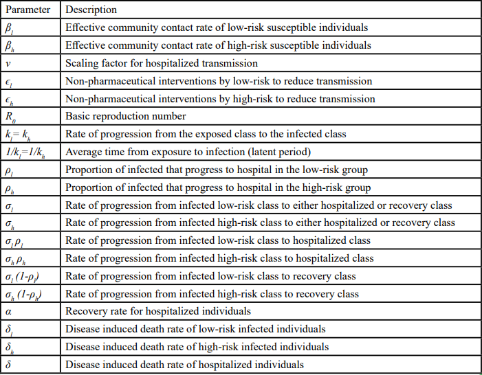
Table 1.
Table 2. Default parameter values used in the deterministic and stochastic models (day⁻¹, unless noted). Parameter values adopted from prior epidemiologic studies and used as fixed inputs for model evaluation [5-7]. These values provide the baseline parameterization for simulations and for fitting procedures used to obtain Table 3.
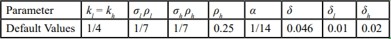
Table 2.
Table 3. Fitted parameter values for Brazil COVID-19 incidence data (first 120 days) and resulting R0. Estimated parameter values obtained by fitting the deterministic model to publicly available Brazil incidence data (Johns Hopkins University) over the first 120 days of the epidemic. The implied basic reproduction number R0 is computed using Eq.(2) under the fitted baseline intervention levels ε1 and εh.

Table 3.
Stochastic Continuous Time Markov Chain
We now introduce stochasticity into the model to capture stochastic variability in epidemic spread. The first step in this process is to recast the deterministic framework as a continuous-time Markov chain (CTMC) [8,9]. This requires enumerating every possible state transition that can occur during an infinitesimal time interval and specifying the corresponding transition probability. Drawing directly from the compartmental structure, the resulting transition types and their associated rates are summarized in Table 4. These rates constitute the infinitesimal generator of the CTMC, which we subsequently use to derive branching-process approximations.
Table 4. CTMC transition types and intensities (infinitesimal generator) for the stochastic epidemic model. All allowable state transitions of the CTMC correspond to the compartmental structure in Figure 1, together with their transition intensities. These intensities define the CTMC generator used for Doob–Gillespie simulation and for deriving the multi-type branching process approximation.
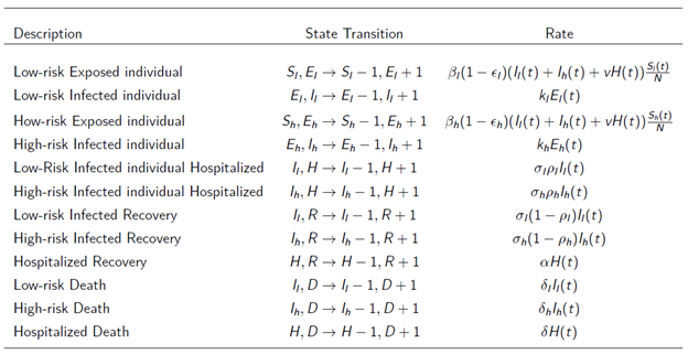
Table 4.
Using the Doob–Gillespie algorithm [10], we generate stochastic realizations of the infected compartments for both high-risk and low-risk subpopulations. The CTMC is calibrated to the Brazilian COVID-19 data with parameter values previously cited. While stochastic fluctuations appear negligible with such a big population size, the variability becomes evident when zooming up the trajectories, or when the model is run for a smaller populations size. To better visualize the differences between the infection trajectories predicted by the deterministic model and those obtained from the stochastic realizations of the CTMC model for both subpopulations, Figure 2 is generated using a smaller population size (N=2,000).
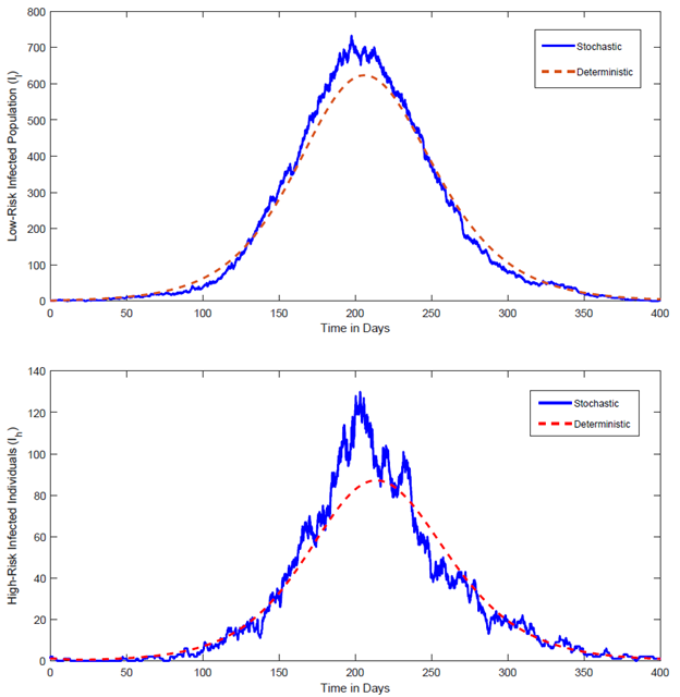
Figure 2. Deterministic infected trajectory versus stochastic CTMC realizations (illustrative reduced population size).
Comparison of the deterministic infected trajectory from system (1) with representative stochastic realizations from the CTMC (simulated via the Doob–Gillespie algorithm) under the same parameterization. For visualization, a reduced population size N is used to make stochastic variability and stochastic extinction events apparent. Curves show stochastic paths fluctuating around the deterministic trajectory; extinction corresponds to paths reaching zero infected individuals.
As illustrated in Figure 2, the stochastic realizations fluctuate above or below the deterministic trajectory, reflecting the inherent randomness in epidemic dynamics in real-world settings. In particular, a fraction of the stochastic paths dies out completely, even when the basic reproduction number R0 > 1; this phenomenon, known as stochastic extinction, is a feature that deterministic models cannot capture.
As shown by the deterministic model, when R0 > 1, deterministic models predict an inevitable epidemic, although earlier interventions can slow the spread, reduce but broaden the peak, and postpone its arrival. In contrast, real-world evidence shows that appropriately sized public-health prevention measures can curb the epidemic even when R0 > 1. Below, we run stochastic simulations to estimate the stochastic extinction probability for R0 > 1 with various combinations of early intervention strength levels in the low-risk and high-risk populations.
Starting from one infectious individual in the high-risk population and none in the low-risk population, the simulated disease extinction probabilities as a function of the health policy intervention parameters for the low-risk group (ϵl) and that for the high-risk group (ϵh), by averaging 10,000 realizations of the CTMC, are shown in Table 5.
In Table 5 and the subsequent Table 6 and Table 7, same as in Figure 4, the values shown in the ϵl and ϵh columns represent multiplicative scaling factors relative to their respective baseline values, rather than the actual parameter values. The baseline values used are ϵl = 0.2729 and ϵh = 0.3432, as specified in Section 2.1. Therefore, for ϵl, the baseline value of 0.2729 corresponds to a scaling factor of 1, while scaling factors of 1.4, 1.6, and 1.8 correspond to actual ϵl values of 0.3821, 0.4366, and 0.4912, respectively. Similarly, for ϵh, the baseline value of 0.3432 corresponds to a scaling factor of 1, and scaling factors of 1.4, 1.6, and 1.8 correspond to actual ϵh values of 0.4805, 0.5491, and 0.6178, respectively. It can be verified easily that for all combinations of ϵl and ϵh values appeared in Tables 5-7, the corresponding basic reproduction number R0 is greater than 1.
Table 5. Estimated extinction probabilities from CTMC simulation under intervention-scaling scenarios (initial seeding in high-risk group).
Estimated epidemic extinction probabilities computed by averaging 10,000 Doob– Gillespie realizations of the CTMC under alternative intervention strengths. Initial condition: one infectious individual in the high-risk group and none in the low-risk group (Ih (0) = 1, Il(0) = 0; other infectious compartments initially zero unless otherwise stated). Columns labeled ϵl and ϵh report multiplicative scaling factors applied to the baseline fitted values in Table 3 (e.g., 1.0 = baseline; 1.4 = 40% increase). For each scenario, R0 > 1.
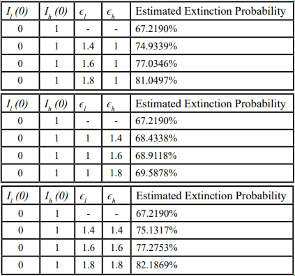
Table 5.
From Table 5, when the epidemic is seeded by a single infectious individual in the high-risk group (and no infection in the low risk group), the stochastic extinction probability under baseline intervention levels (ϵl = 0.2729, ϵh = 0.3432 R0 = 1.4017), is roughly 67%. Increasing either ϵl, or ϵh, or both raises the extinction probability, but the magnitude of the effect differs substantially. Specifically, increasing ϵh alone leads to a slight improvement in the extinction probability, whereas an equivalent proportional increase in ϵl produces a much larger rise in the extinction probability, nearly matching the impact of increasing both ϵl and ϵh simultaneously at the same scale.
For example, when ϵl is held at its baseline and ϵh is increased to 1.4 × baseline (a 40% increase from its baseline value), the extinction probability increases only from roughly 67% to about 68%. In contrast, when ϵl = 1.4 × baseline (with ϵh at its baseline value), or when both ϵl and ϵh are increased to 1.4 × baseline, the extinction probability rises to roughly 75%.
These results indicate that even when the epidemic originated solely in the high-risk subpopulation, strengthening interventions in the low-risk groups can yield an extinction probability comparable to that achieved by intensifying interventions of the same scale to both groups. By contrast, focusing exclusively on the high-risk group produces a substantially lower likelihood of disease extinction.
In the following section, we discuss how to estimate the probability of stochastic extinction using a branching process approximation.
Multi-type branching process approximation
An analytical approach of estimating the probability of stochastic extinction can be obtained from branching process theory. The idea of branching processes dates back to the French actuary Irenée-Jules Bienaymé, whose 1845 paper “On the Law of Multiplication and the Duration of Families” [11] anticipated the well-known Bienaymé-Galton-Watson (BGW) branching process. The original BGW model was devised to study the extinction of family names under the assumption that surnames are transmitted solely from father to son, and all men have the same probability of having 0, 1, 2, … sons reaching adulthood. Thus, a family name becomes extinct when all male descendants die without adult male heirs. After a period of dormancy, research on branching processes revived in the early 20th century and expanded substantially after World War II. In this study, we employ a multi-type branching process to approximate our stochastic epidemic model.
Specifically, in our CTMC model, five infectious compartments are considered:
• Class 1: low-risk exposed individuals (El)
• Class 2: low-risk infectious individuals (Il)
• Class 3: high-risk exposed individuals (Eh)
• Class 4: high-risk infected individuals (Ih)
• Class 5: Hospitalized individuals (H)
Accordingly, in the multi-type branching process framework, the process is represented as
V(t)=(El(t), Il(t), Eh(t), Ih(t), H (t)),
where El(t), Il(t), Eh(t), Ih(t) and H (t) denote the numbers of individuals in the corresponding infectious class at time t. The offspring distribution can be derived directly from the state transition rates provided in Table 4. Because each transition is Poisson in continuous time, the numbers of offspring of the five types are independent Poisson variables with means equal to the corresponding rates divided by the total exit rate of the parent.
For each type i (i = 1, 2,…,5), we define the probability-generating function (pgf),
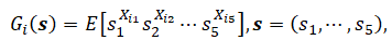
equation 3
where Xij is the number of type-j offspring produced by a single type-i. The vector π = ( π1,..., π5) satisfies the fixed-point system

equation 4
The overall extinction probability for an arbitrary initial state k = (k1,..., k5) is then
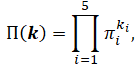
equation 5
i.e. the product of the single-type extinction probabilities raised to the number of initial individuals of each type.
Hence, let El(0), Il(0), Eh(0), Ih(0), H (0) denote the initial counts of individuals across the five infectious classes, and 0 =(0,0,0,0,0), the overall extinction probability is

equation 6
Results
Deterministic baseline dynamics
Asempapa, R. et al [1] demonstrated that the cumulative COVID-19 cases predicted by this compartmental model for the first 120 day of the epidemic in Brazil match the reported data closely, with only minor random deviations. This concordance validates the model as a robust baseline for embedding stochastic components that capture random fluctuations.
As we can see in Table 3, for the COVID-19 outbreak in Brazil, the estimated value of the basic reproduction number is R0 = 1.4. This means that, on average, each infectious individual transmits the disease to roughly 1.4 others, so the epidemic is expected to grow, making an outbreak unavoidable under the baseline non-pharmaceutical intervention levels in the low-risk and high-risk groups ϵl = 0.2729 and ϵh = 0.3432, respectively.
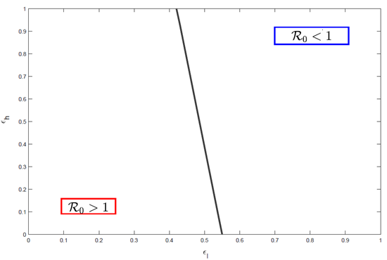
Figure 3. Basic reproduction number R0 as a function of intervention strengths in the low-risk and high-risk groups
Contour plot of R0 computed from Eq. (2) across values of the intervention parameters ϵl (low-risk) and ϵh (high-risk), holding all other parameters fixed at baseline/fitted values (Tables 2–3). The threshold R0 = 1 is indicated to delineate deterministic growth versus decline.
Though equation (2) shows that, holding all other parameters constant, R0 is a linear combination of ϵl and ϵh, and Figure 3 illustrates how these two interventions rates influence R0. The results highlight that the non-pharmaceutical intervention level in the low-risk group, ϵl, is the decisive factor for disease extinction. Specifically:
• When ϵl < 0.41: no degree of interventions in the high-risk group can reduce R0 below 1, implying that the disease will persist regardless of efforts targeted solely at the high-risk population.
• When ϵl > 0.55: R0 can fall below 1 even in the absence of interventions in the high-risk group, ensuring that the disease will eventually die out.
Solutions to the deterministic model (1) also depend on ϵl and ϵh. Holding all other parameters at their values listed in Tables 2 and 3, and specifically, ϵh is fixed at its baseline value of 0.3432, Figure 4 illustrates how the Susceptible and Exposed populations evolve in both the low-risk and high-risk populations as ϵl varies. Here, the baseline value of ϵl is 0.2729 (as listed in Table 3), and numbers in the legend denote multiplicative factors relative to this baseline (for example, “(0.5) baseline” means ϵl = 0.5 × 0.2729 = 0.1365). Thus, multipliers less than 1 represent relaxed health prevention measures, whereas multipliers greater than 1 indicate stricter health intervention policies compared to the default baseline intervention conditions.
Deterministic solutions of system (1) showing the evolution of susceptible and exposed populations in the low-risk and high-risk subpopulations as ϵl varies by multiplicative factors relative to its baseline fitted value (Table 3), while holding ϵh fixed at its baseline fitted value. Legend entries denote the multiplier applied to baseline ϵl (e.g., 1.0 = baseline). All other parameters are fixed at Tables 2–3.
The trajectories in Figure 4 reveal that stronger interventions in the low-risk population (higher ϵl) slow the decline of the susceptible population, reduce the magnitude of the exposed (and thus infected) peak, and delay the peak’s occurrence in both the low-risk and high-risk subpopulation. Conversely, weaker interventions (smaller ϵl) accelerate the depletion of susceptible individuals and yield a higher and earlier exposed (and thus infected) peak in both groups. When ϵl is increased to 1.8 times its baseline value, the susceptible population in both the low-risk and high-risk groups remains nearly constant, and the disease exerts minimal impact on either subpopulation.
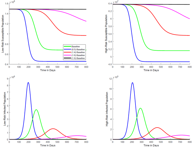
Figure 4. Deterministic trajectories under varying low-risk intervention strength ϵl (Brazil parameterization).
Stochastic extinction probabilities and scenario comparisons
In this section, we evaluate the stochastic extinction probabilities for the two different initial scenarios mentioned in the Methods section. The purpose is twofold: to validate the branching-process calculations against the numerical simulation of the CTMC, and to explore how extinction probabilities change under alternative initial conditions and different levels of interventions.
As mentioned previously, all parameter combinations listed in Tables 6–7 satisfy R0 > 1, thus the deterministic models predict an inevitable outbreak. Nevertheless, the stochastic framework reveals non-zero extinction probabilities.
First, we consider the case discussed in the baseline initial condition: a single initially infected individual occurs in the high-risk population and no infections in the low-risk population. In the baseline initial condition, the stochastic extinction probabilities were estimated by averaging 10,000 Gillespie realizations of the CTMC model for each combination of ϵl and ϵh values. Here, we compute the extinction probabilities directly from the fixed-point system (3). These results are summarized in Table 6.
From Table 6, it is evident that the extinction probabilities obtained using two approaches are very close, confirming the reliability of both. These findings further support the conclusion presented in the baseline initial condition: even when the single initial infection occurs in the high-risk group and the low-risk group has no infections, implementing stricter non-pharmaceutical interventions in the low-risk group alone is nearly as effective as applying them to both groups, and substantially more effective than targeting only the high-risk group.
Table 6. Validation of extinction probabilities: CTMC simulation versus branching-process calculation (initial seeding in high-risk group). Comparison of extinction probabilities estimated by CTMC simulation (10,000 Gillespie realizations) versus extinction probabilities computed from the multi-type branching process fixed-point equations under the same intervention-scaling scenarios. Initial condition corresponds to Table 5 (Ih (0)=1, I1 (0)= 0). Scaling factors in ε1 and εh are relative to baseline fitted values in Table 3.
Table 7 shows similar patterns to those observed in the first scenario regarding how the level of non-pharmaceutical interventions in the low-risk and high-risk groups (ϵl and ϵh, respectively) influence the stochastic disease extinction probabilities. Specifically, under baseline intervention levels for both groups (ϵl = 0.2729, ϵh = 0.3432, R0 = 1.4017), the estimated stochastic disease extinction probability for this scenario is approximately 68%. As the strength of non-pharmaceutical interventions increases in either group or both groups, the extinction probability rises accordingly. However, the magnitude of the impact on the extinction probability differs between ϵl and ϵh. Once again, applying stricter interventions in the low-risk population alone achieves nearly the same extinction probability as applying them to both populations, and performs markedly better than focusing interventions exclusively on the high-risk population.
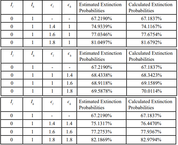
Table 6.
Table 7. Extinction probabilities under alternative initial seeding (initial infection in low-risk group): simulation versus branching-process calculation. Extinction probabilities estimated by CTMC simulation (10,000 Gillespie realizations) and computed using the branching-process approximation under alternative intervention- scaling scenarios. Initial condition: one infectious individual in the low-risk group and none in the high-risk group (I1(0)=1, Ih(0)=0; other infectious compartments initially zero unless otherwise stated). Scaling factors in ε1 and εh are relative to baseline fitted values in Table 3; for each scenario, R0 > 1.
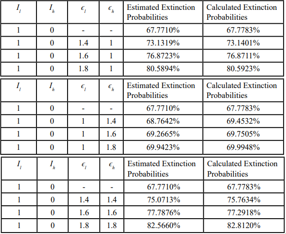
Table 7.
Discussion
Extinction probability provides a decision-relevant complement to deterministic metrics such as the basic reproduction number. In early epidemic phases, when case counts are low, random variation in contacts and transmission can produce a non-trivial chance of fade-out even when a deterministic model with fitted parameters implies growth (R0 > 1). By embedding a continuous-time Markov chain (CTMC) within a standard compartmental framework and approximating early dynamics using a multi-type branching process, we quantify how alternative intervention strengths shift the chance that transmission chains terminate before sustained epidemic growth occurs.
These results fit within the broader public health modeling literature. Deterministic compartmental models remain essential for describing average trajectories and for interpreting how parameters shape dynamics [2-4]. However, stochastic epidemic models are required to characterize extinction versus major outbreak outcomes when infections are sparse, and CTMC formulations and branching-process approximations provide standard tools for this purpose [5,6]. In the COVID-19 context, early estimates of transmission potential and analyses of non-pharmaceutical interventions underscore that growth conditions alone do not determine realized outcomes and that timely suppression of community transmission can materially change epidemic trajectories [8-10].
A central finding is that proportional strengthening of non-pharmaceutical interventions in the low-risk subpopulation produces substantially larger gains in extinction probability than an equivalent proportional increase confined to the high-risk subpopulation. This pattern is consistent with the principle that suppressing transmission in the larger transmitting group reduces the force of infection experienced by all subpopulations, including high-risk individuals, thereby increasing the likelihood of early fade-out even when the outbreak is initially seeded in the high-risk group.
From a public health implementation standpoint, the results emphasize broad measures that reduce effective contacts and improve adherence in settings that drive transmission. For respiratory epidemics, actionable levers include reducing crowding in high-contact venues, improving indoor air quality, promoting masking during periods of elevated risk, enabling rapid access to testing and isolation, and supporting adherence through clear risk communication and practical resources that make compliance feasible. Targeted protections for high-risk groups remain essential for reducing severe outcomes, but our results indicate that high-risk-only strategies are unlikely to maximize the probability of extinction when substantial transmission potential persists in the broader community.
Finally, the close agreement between extinction probabilities estimated via Monte Carlo CTMC simulation and those computed from the branching-process fixed-point system supports the internal validity of the analytic approximation under the early-epidemic conditions considered. Practically, extinction probability can be used as an explicit endpoint to compare candidate intervention packages, to justify early population-level measures when elimination remains feasible, and to communicate probabilistic benefits to decision-makers when deterministic predictions alone suggest inevitable growth.
Limitations
This work has several limitations that should be considered when interpreting the findings and translating them to policy.
• The branching-process approximation is most accurate during the early outbreak phase; accuracy may diminish as susceptible depletion becomes substantial or as behavioral responses and time-varying interventions alter transmission dynamics over time.
• The model assumes homogeneous mixing within and between the low-risk and high-risk groups. Real-world contact patterns are heterogeneous and structured by age, household composition, occupation, geography, and network effects, which could change the relative impact of targeted versus population-wide interventions.
• Interventions are represented through constant multiplicative reductions in effective transmission. In practice, NPIs are implemented and relaxed over time, adherence varies across individuals and settings, and enforcement and risk perception change dynamically.
• Parameter uncertainty is not fully propagated. Parameters are estimated from early-epidemic incidence data, and different parameter combinations can produce similar fitted trajectories, which can affect derived extinction probabilities and comparisons between scenarios.
• The analysis uses publicly available, aggregated incidence data. Such data can be affected by reporting delays, under-ascertainment, changes in testing capacity and case definitions, and temporal aggregation, particularly during the first months of an epidemic.
• The model does not explicitly incorporate vaccination, variants, therapeutics, imported cases, or spatial spread. Therefore, results are most directly applicable to early-stage outbreaks in largely susceptible populations under relatively stable transmission conditions.
Public Health Significance and Policy Implications and Recommendations
These results support several actionable public health implications for early outbreak response, particularly when elimination remains feasible and surveillance indicates low-to-moderate incidence.
First, intervention packages intended to increase the probability of extinction should prioritize measures that reduce transmission broadly in the community, especially those that improve compliance or reduce contacts in the larger low-risk group. Examples include interventions in high-contact environments (workplaces, schools, and mass gatherings), clear risk communication and adherence support, and rapid testing and isolation infrastructure that enables early interruption of transmission chains.
Second, targeted protections for high-risk groups should be implemented in parallel to reduce morbidity and mortality, but they should be viewed as insufficient on their own for maximizing extinction probability when substantial transmission potential persists in the broader community.
Third, extinction probability can be operationalized as a decision metric alongside R0 and incidence trends. Agencies can use the framework to compare candidate non-pharmaceutical intervention packages by quantifying how much each package increases the chance of elimination over a defined time horizon, thereby enabling transparent comparison of intervention intensity versus expected benefit.
Finally, these findings underscore the value of timeliness. When incidence is low, short, decisive population-wide measures may yield disproportionately large gains in extinction probability relative to later implementation, when transmission chains are numerous and stochastic fade-out is less likely.
• Use extinction probability to rank candidate non-pharmaceutical intervention packages during the early response window, rather than relying on R0 alone.
• Prioritize population-wide transmission suppression measures that are feasible to implement rapidly and that sustain high adherence in the broader low-risk population.
• Maintain targeted protections for high-risk groups to reduce severe outcomes, but avoid relying exclusively on high-risk-only interventions to achieve elimination.
Conclusion
Although when the basic reproduction number exceeds 1, the deterministic model alone would forecast an inevitable epidemic, our incorporation of stochasticity through a CTMC and a multi-type branching process approximation, demonstrates that non-pharmaceutical interventions can still produce a non-negligible probability of disease extinction, in line with empirical observations.
The analysis pinpoints compliance in the low-risk subpopulation as the key lever for maximizing extinction probability. Strategies that focus solely on the high-risk group are insufficient; in contrast, elevating intervention levels in the low-risk subpopulation yields substantially greater benefits. While strengthening interventions in both subpopulations provides the highest extinction probability, the improvement is nearly comparable to targeting the low-risk group alone.
These findings underscore the importance of stochastic modeling for public-health decision-making and suggest that, in future outbreaks, resources should be directed preferentially toward broad, population- wide interventions, especially those aimed at the low-risk group, to maximize the likelihood of epidemic control.
Conflict of Interest Statement:
The authors have no conflicts of interest to disclose.
Author Contributions
All authors contributed equally to all aspects of this manuscript. All authors approved the final manuscript and agree to be accountable for all aspects of the work.
Ethics Approval/Consent
IRB review and informed consent were not required because the study used publicly available, de-identified, aggregated incidence data.
Funding Statement
The authors received no internal or external funding for this work.
Data Availiability Statement
All data used in this study are publicly available, de-identified, aggregated incidence data.
References
Asempapa, R., Oduro, B., Apenteng, O. O. & Magagula, V. M. A COVID-19 mathematical model of at-risk populations with non-pharmaceutical preventive measures: The case of Brazil and South Africa. Infect. Dis. Model. 7, 45–61 (2021). View
Blackwood, J. C. & M.Childs, L. (2018). An introduction to compartmental modeling for the budding infectious disease modeler. Lett. Biomath. 5, 195–221. View
Hamer, W. H. (1906). The Milroy Lectures on Epidemic Disease in England — The Evidence of Variability and of Persistency of Type. The Lancet, 167, 569–574. View
Brauer, F. (2017). Mathematical epidemiology: Past, present, and future. Infect. Dis. Model. 2, 113–127. View
Li, Q. et al. (2020). Early Transmission Dynamics in Wuhan, China, of Novel Coronavirus–Infected Pneumonia. N. Engl. J. Med. 382, 1199–1207. View
Tang, B. et al. (2020). Estimation of the Transmission Risk of the 2019- nCoV and Its Implication for Public Health Interventions. J. Clin. Med. 9, 462. View
Ferguson, N. et al. (2020). Report 9: Impact of non-pharmaceutical interventions (NPIs) to reduce COVID-19 mortality and healthcare demand. View
Allen, L. J. S. (2017). A primer on stochastic epidemic models: Formulation, numerical simulation, and analysis. Infect. Dis. Model. 2, 128–142. View
Lahodny Jr., G. E., Gautam, R. & Ivanek, R. (2015). Estimating the probability of an extinction or major outbreak for an environmentally transmitted infectious disease. J. Biol. Dyn. 9, 128–155. View
Gillespie, D. T. (1976). A general method for numerically simulating the stochastic time evolution of coupled chemical reactions. J. Comput. Phys. 22, 403–434. View
Bienaymé, J. (1845). De la loi de multiplication et de la durée des familles. Soc Philomat. Paris Extraits, 13, 131-132. View