
- About the Journal
- Editorial Board
- Review Process
- Author Guidelines
- Article Processing Charges
- Special Issues
- Current Issue
- Past Issue
 Contributions to Pure and Applied Mathematics
Contributions to Pure and Applied Mathematics Volume 1 (2023), Article ID: CPAM-105
https://doi.org/10.33790/cpam1100105Research Article
Unique Continuation for the Multi-term Time Fractional Diffusion Equation and its Numerical Simulation
Yuanyuan Yang1, Lejiao Zhao2, Zhiyuan Li3
1,2Hebei Vocational University of Technology and Engineering, China
3*Ningbo University, China
Corresponding Author Details: Yuanyuan Yang, Professor, Department of Mathematics and Statistics, Ningbo University, China.
Received date: 25th October, 2023
Accepted date: 25th November, 2023
Published date: 08th December, 2023
Citation: Yang, Y., Zhao, L., and Li, Z.,(2023). Unique Continuation for the Multi-Term Time Fractional Diffusion Equation and its Numerical Simulation. Contrib Pure Appl Math, 1(1): 105. doi: https://doi.org/10.33790/cpam1100105.
Copyright: ©2023, This is an open-access article distributed under the terms of the Creative Commons Attribution License 4.0, which permits unrestricted use, distribution, and reproduction in any medium, provided the original author and source are credited.Creative Commons Attribution License, which permits unrestricted use, distribution, and reproduction in any medium, provided the original author and source are credited
Abstract
This paper deals with the unique continuation principle of solutions for a one-dimensional anomalous diffusion equation with multi-term time fractional derivatives. The proof is mainly based on the Laplace transform and Theta function method. Numerically, we reformulate the unique continuation as an optimization problem, and propose an iterative thresholding algorithm to simulate it numerically. Finally, several numerical experiments are presented to show the accuracy and efficiency of the algorithm.
Introduction and main results
In this paper, letting \(T>0\), \(\ell\in\mathbb N^+\) and \(\alpha_j,q_j\) (\(j=1,2,\ldots,\ell\)) be positive constants such that \(0<\alpha_\ell<\cdots<\alpha_1<1\), we consider the following one-dimensional time-fractional diffusion equation with multi-term time fractional derivatives \[\label{eq-gov} \sum_{j=1}^\ell q_j \partial_t^{\alpha_j }u(x,t) - \partial_x^2 u(x,t) = 0, \quad (x,t)\in(0,1)\times(0,T].\] (1.1) Here by \(\partial_t^{\alpha_j}\) we denote the Caputo derivative (see, e.g., Podlubny [17 2.4.1]) \[\partial_t^{\alpha_j}g(t):=\frac1{\Gamma(1-\alpha_j)}\int_0^t\frac{g'(\tau)}{(t-\tau)^{\alpha_j}}\,d\tau,\quad t>0,\] where \(\Gamma(\,\cdot\,)\) stands for the Gamma function.
Unlike the usual parabolic equations characterized by exponential decay in time and Gaussian profile in space, fractional diffusion equations possess properties of slow decay in time and long-tailed profile in space. Therefore, fractional diffusion equations are more suitable model equations than parabolic equations for modeling anomalous diffusion with non-Fickian growth rates and long-tailed profiles (see e.g., Adams and Gelhar [1] and Hatano and Hatano [6]. Theoretical research has developed rapidly, and it has been proven that most properties of parabolic equations, such as well-posedness, (Strong) Maximum principle, analyticity, and asymptotic behavior, have been parallelly extended to the fractional order case. see, e.g., Liu, Rundell and Yamamoto [14], Luchko [15], Sakamoto and Yamamoto [19] for the single-term time fractional diffusion equations (that is \(\ell=1\)). For the multi-term case, one can refer to Li, Liu and Yamamoto [9], Liu [12], Luchko [16] and the references therein.
In addition to the aforementioned aspects, the unique continuation principle (UCP) is also one of the remarkable characteristics of parabolic equations. In recent years, there has been increasing interest in extending this theory to fractional order equations, given their widespread application in various areas of science and engineering. For example The UCP was used to solve the uniqueness of some inverse problems on determining the spatially dependent component of the sources [7, 13, 20] and the references there in). Not only for the inverse problems but also for the approximate control problems, one of the very important key in dealing with these problems is the UCP, see e.g., Fujishiro and Yamamoto [5]
To the best knowledge of the authors, the UCP for the multi-term case has not yet been established. With this in mind, we aim to generalize this property to the fractional case. Building on Laplace transforms and fractional Theta functions, we have
Theorem 1. Let \(I\) be a nonempty open subinterval of \((0,1)\) and \(2\alpha_\ell>\alpha_1\). We suppose \(u\in L^2(0,T;H^2(0,1))\) is a solution to the fractional diffusion equation (1.1). Then \(u=0\) in \((0,1)\times(0,T)\) provided that \(u\equiv0\) in \(I\times[0,T]\).
Uniqueness result similar to Theorem 1 was established in Li and Yamamoto [10], where the one-dimensional time-fractional discussion equation was studied, and the uniqueness of solutions was shown using the Theta function method. For the general case of multiple dimensions, there is currently no positive answer regarding the UCP. However, under some addition assumptions on the solutions, one can still obtain similar uniqueness results. We refer to Jiang, Li, Liu and Yamamoto [7] and Sakamoto and Yamamoto [19] in which the homogeneous Dirichlet boundary condition on the entire boundary was required and the existence of eigensystem provides convenience for the argument. On the other hand, in the case of the homogeneous initial condition, the UCP was proved in Cheng, Lin and Nakamura [3] for half-order fractional diffusion equation using Carleman estimates for the operator \(\partial_t-\triangle^2\). For a general fractional order in the \((0,1)\) interval, Lin and Nakamura [11] recently established the UCP by applying a newly developed Carleman estimate based on calculus of pseudo-differential operators.
The remainder of this paper is organized as follows. In Section 2, we introduce all necessary background information about the fundamental solution of (1.1) and the fractional Theta function. Then, Section 3 is devoted to the proof of the main theorem. In Section 4.1, we propose an iterative thresholding algorithm for numerically simulating the UCP of the solution. This is followed by several numerical examples in Section 4.2 that illustrate the performance of the proposed method. Finally, a concluding remark is given in Section 5.
Preliminary material
Fundamental solution
Let \(K(x,t)\) be the fundamental solution of the following free space-time fractional diffusion equation \[\label{eq-free} \left\{ \begin{alignedat}{2} &\sum_{j=1}^\ell q_j \partial_t^{\alpha_j }K(x,t) = \partial_x^2 K(x,t), &\quad& x\in{\rm \mathbb R},\ t>0, \\ &K(x,0)=\delta(x), &\quad& x\in{\rm \mathbb R} ---------- (2.1), \end{alignedat} \right.\] where we denote \(\delta(x)\) as the Dirac delta function. We consider the Laplace transform of the fundamental solution \(K(x, t)\) with respect to time variable \(t\). For this, we apply Laplace transform on both sides of the equation \((2.1)\) and then \[\left\{ \begin{alignedat}{2} &\sum_{j=1}^\ell q_j s^{\alpha_j} \widehat K(s) =\partial_x^2 \widehat K(s) + \sum_{j=1}^\ell q_j s^{\alpha_j-1}\delta(x), \\ &K(x,0)=\delta(x), \quad x\in\mathbb R. \end{alignedat} \right.\] Then taking Fourier transform \(\mathcal{F}\), and noting that the formula \(\mathcal F[\delta] = 1\) and \(\mathcal F[\partial_x^2 K](\xi) = -\xi^2 \mathcal F[K](\xi)\), we see that \[\sum_{j=1}^\ell q_j s^{\alpha_j} \mathcal{F}[\widehat K(s)] =-\xi^{2}\mathcal{F}[\widehat K(s)] + \sum_{j=1}^\ell q_j s^{\alpha_j-1}.\] We denote \(\phi(s):=\sum_{j=1}^\ell q_j s^{\alpha_j}\), then we can rephrase the above therm as follows \[\phi(s) \mathcal{F}[\widehat K(s)] =-\xi^2\mathcal{F}[\widehat K(s)] + s^{-1} \phi(s).\] Therefore \[\mathcal{F}[\widehat K(s)](\xi) = \frac{s^{-1}\phi(s)}{\phi(s)+\xi^2}.\] Using the Fourier inverse transform, we obtain the Laplace transform \(\widehat K\) of the fundamental solution to (2.1) \[\widehat K(s) =\mathcal{F}^{-1}\left[\frac{s^{-1}\phi(s)}{\phi(s)+\xi^2}\right] =\frac{1}{2\pi}\int_{-\infty}^\infty e^{ix\xi} \frac{s^{-1}\phi(s)}{\phi(s)+\xi^2} d\xi.\] We next calculate the complex integral \(\mathcal{F}^{-1}\left[\frac{s^{-1}\phi(s)}{\phi(s)+\xi^2}\right]\).
Lemma 2.1.
\[\mathcal{F}^{-1}\left[\frac{s^{-1}\phi(s)}{\phi(s)+\xi^2}\right](x) =\frac1{2s} \phi^\frac12(s) \exp\{-\phi^{\frac12}(s)|x|\}.\]
Proof.
Proof. From the inverse Fourier transform formula, we have \[\mathcal{F}^{-1}\left[\frac{s^{-1}\phi(s)}{\phi(s)+\xi^2}\right](x) =\frac{1}{2\pi}\int_{-\infty}^\infty e^{ix\xi} \frac{s^{-1}\phi(s)}{\phi(s)+\xi^2} d\xi.\] We denote the contour from \(-R\) to \(R\) by \(C_{0}\), the semicircle with radius \(R\) in the upper and lower half plane by \(C_{R^{+}}\) and \(C_{R^{-}}\) respectively. Also let \(C_{+}\),\(C_{-}\) be the closed contours which consist of \(C_{0}\),\(C_{R^{+}}\) and \(C_{0}\),\(C_{R^{-}}\) respectively.
For the case of \(x>0\),working on the closed contour \(C_{+}\), we have \[\begin{aligned} \frac{1}{2\pi}\int_{-\infty}^\infty e^{ix\xi} \frac{s^{-1}\phi(s)}{\phi(s)+\xi^2} d\xi &=\lim_{R\rightarrow+\infty} \frac{1}{2\pi}\oint_{C_{+}}e^{ix\xi} \frac{s^{-1}\phi(s)}{\phi(s)+\xi^2} d\xi -\lim_{R\rightarrow+\infty}\frac{1}{2\pi}\int_{C_{R^{+}}}e^{ix\xi} \frac{s^{-1}\phi(s)}{\phi(s)+\xi^2} d\xi \\ &=\lim_{R\rightarrow+\infty}\frac{1}{2\pi}\oint_{C_{+}}e^{ix\xi} \frac{s^{-1}\phi(s)}{\phi(s)+\xi^2} d\xi , \end{aligned}\] where the second limit is 0 as follows from Jordan’s Lemma. Since \(0<\alpha_j <1\) and \(q_j >0\), by our assumption, we have \(\Re \phi(s) = \sum_{j=1}^\ell q_j |s|^{\alpha_j } \cos\alpha_j \theta\geq0\), which in turns leads to \(\Re \phi^{\frac12}(s)\geq0\).
Then there is only one singular point \(\xi=i\phi^{\frac12}(s)\) in \(C_{+}\) which is continued by the upper half plane. By the residue theorem, we have \[\begin{aligned} \lim_{R\rightarrow+\infty}\frac{1}{2\pi}\oint_{C_{+}}e^{ix\xi} \frac{s^{-1}\phi(s)}{\phi(s)+\xi^2} d\xi &=\lim_{R\rightarrow+\infty}2\pi i\frac{1}{2\pi} \exp \left\{ ix(i \phi^{\frac12}(s)) \right\} \frac{s^{-1} \phi(s)}{2 i\phi^{\frac12}(s)} \\ &=\frac1{2s} \phi^{\frac12}(s) \exp\left\{ -\phi^{\frac12}(s) x \right\}. \end{aligned}\] For the case of \(x<0\), similarly, we have \[\frac{1}{2\pi}\int_{-\infty}^\infty e^{ix\xi} \frac{s^{-1}\phi(s)}{\phi(s)+\xi^2} d\xi =\frac1{2s} \phi^{\frac12}(s) \exp\left\{ \phi^{\frac12}(s) x \right\}.\] Therefore, \[\mathcal{F}^{-1}\left[\frac{s^{-1}\phi(s)}{\phi(s)+\xi^2}\right](x) =\frac1{2s} \phi^{\frac12}(s) \exp\left\{ -\phi^{\frac12}(s) |x| \right\},\] which completes the proof of the lemma. ◻
From the above lemma, it follows that the fundamental solution \(K(x,t)\) has the following formula of the Laplace transform with respect to \(t\), \[\widehat{K}(x,s) =\frac{\phi^{\frac12}(s)}{2s}\exp\left\{-\phi^{\frac12}(s)|x| \right\},\quad x\in\mathbb R,\ \phi(s)=\sum_{j=1}^\ell q_j s^{\alpha_j }.\]
Lemma 2.2.
The functions \(K(x,t)\) is even with respect to \(x\) and satisfies the following estimates \[\label{esti-theta<1} |K(x,t)| \le C \sum_{j=1}^\ell t^{-\frac{\alpha_j}2},\quad (x,t)\in\mathbb R\times(0,\infty),\]---------(2.2) and for the Riemann-Liouville derivative \(D_t^{1-\alpha} K(x,t)\) with \(\alpha>\frac{\alpha_1}2\): \[\label{esti-theta'<1} |D_t^{1-\alpha} K(x,t)| \le C \sum_{j=1}^\ell t^{\alpha-\frac{\alpha_j}2-1},\quad (x,t)\in\mathbb R\times(0,\infty),\]----------(2.3) where the constant \(C>0\) is independent of \(t\), but may depend on \(\alpha\), \(\{\alpha_j\}_{j=1}^\ell\).
Proof. From the Laplace transform of \(K(x,t)\):
\[\widehat{K}(x,t)=\frac12 s^{-1}
\phi^{\frac12}(s) \exp\left\{-\phi^{\frac12}(s)|x| \right\},\] we
conclude from the Fourier-Millin formula (e.g., Schiff [22]) for the inversion Laplace
transform that \(K(x,t)=\mathcal
L^{-1}[\widehat K(s)]\) admits \[K(x,t)=\frac{1}{4\pi
i}\int_{\gamma-i\infty}^{\gamma+i\infty}
s^{-1}{\phi^{\frac12}(s)}\exp\left\{-\phi^{\frac12}(s)|x|
\right\}e^{st}ds,\] where \(\gamma>0\) is any fixed constant, from
which we can directly derive the following estimate \[|K(x,t)|\leq\frac{1}{4\pi}
\int_{\gamma-i\infty}^{\gamma+i\infty} |s|^{-1} |\phi^{\frac12}(s)|
\exp\left\{-\frac{\sqrt{2}}{2}|\phi^{\frac12}(s)||x| \right\}|
ds|e^{\gamma t}.\] Moreover, from the definition of \(\phi(s)\), we see that \[|\phi(s)|\geq\sum_{j=1}^\ell
q_{j}|s|^{\alpha_{j}}\cos\alpha_{j}\theta
\geq\sum_{j=1}^\ell q_{j}|s|^{\alpha_{j}}\cos\alpha_{j}\frac{\pi}{2}
\geq c_{0}\sum_{j=1}^\ell |s|^{\alpha_{j}},\] where \(c_{0}:=\min\limits_{1\leq j\leq
\ell}\{q_{j}\cos\frac{\alpha_{j}}{2}\pi\}.\) Therefore, \[\begin{aligned}
|K(x,t)|
&\leq\frac{1}{4\pi}
\int_{\gamma-i\infty}^{\gamma+i\infty} |s|^{-1}\left( \sum_{j=1}^\ell
q_{j}|s|^{\alpha_{j}} \right)^{\frac12}
\exp\left\{-\frac{\sqrt{2}}{2}c_{0}^{\frac12} \left( \sum_{j=1}^\ell
|s|^{\alpha_{j}} \right)^{\frac12}|x| \right\}|ds|e^{\gamma t}\\
&\leq\frac{\left(\max\{q_{j}\} \right)^{\frac12}}{4\pi}
\int_{\gamma-i\infty}^{\gamma+i\infty} |s|^{-1} \left(
\sum_{j=1}^\ell|s|^{\alpha_{j}} \right)^{\frac12}
\exp\left\{-\frac{\sqrt{2}}{2}|x|c_{0}^{\frac12} \left(
\sum_{j=1}^\ell|s|^{\alpha_{j}} \right)^{\frac12} \right\}|ds|e^{\gamma
t}.
\end{aligned}\] For short, we denote \(c_1:=\frac{\sqrt{2}}{2}c_{0}^{\frac12}\)
and nothing that \(s=\gamma+i\eta\),
\(\eta\in(-\infty,+\infty)\), we have
\[\begin{aligned}
|K(x,t)|
&\leq\frac{(\max\{q_{j}\})^{\frac12}}{4\pi}
\int_{-\infty}^\infty
\frac{\left[\sum_{j=1}^\ell(\gamma^{2}+\eta^{2})^{\frac{\alpha_{j}}{2}}
\right]^{\frac12}}
{(\gamma^{2}+\eta^{2})^{\frac12}} \exp\left\{-c_1|x|
\left[\sum_{j=1}^\ell
(\gamma^{2}+\eta^{2})^{\frac{\alpha_{j}}{2}} \right]^{\frac12}\right\}
d\eta e^{\gamma t}\\
&=\frac{\max\{q_{j}^{\frac12}\}}{2\pi}
\int_0^\infty \frac{\left[
\sum_{j=1}^\ell(\gamma^{2}+\eta^{2})^{\frac{\alpha_{j}}{2}}
\right]^{\frac12}}
{(\gamma^{2}+\eta^{2})^{\frac12}} \exp\left\{-c_1|x|\left[
\sum_{j=1}^\ell
(\gamma^{2}+\eta^{2})^{\frac{\alpha_{j}}{2}} \right]^{\frac12}\right\}
d\eta e^{\gamma t}\\
&=\frac{\max\{q_{j}^{\frac12}\}}{2\pi}
\int_0^\infty
\left[\sum_{j=1}^\ell(\gamma^{2}+\eta^{2})^{\frac{\alpha_{j}}{2}-1}
\right]^{\frac12}
\exp\left\{-c_1|x| \left[ \sum_{j=1}^\ell
(\gamma^{2}+\eta^{2})^{\frac{\alpha_{j}}{2}} \right]^{\frac12}\right\}
d\eta e^{\gamma t}.
\end{aligned}\] By changing the variable \(\eta/\gamma\) to \(\eta\), we find \[\begin{aligned}
|K(x,t)|
\le\frac{\max\{q_{j}^{\frac12}\}}{2\pi}
\int_0^\infty \left[
\sum_{j=1}^\ell(1+\eta^{2})^{\frac{\alpha_{j}}{2}-1} \gamma^{\alpha_j}
\right]^{\frac12}
\exp\left\{-c_1|x| \left[ \sum_{j=1}^\ell
(1+\eta^{2})^{\frac{\alpha_{j}}{2}}
\gamma^{\alpha_j}\right]^{\frac12}\right\}
d\eta e^{\gamma t}.
\end{aligned}\] We divide the integral on the right-hand side of
above inequalities into two parts: \[\begin{aligned}
&|K(x,t)|
\\
\leq&\frac{\max\{q_{j}^{\frac12}\}}{2\pi}
\int_{0}^{1}\left[\sum_{j=1}^\ell(1+\eta^{2})^{\frac{\alpha_{j}}{2}-1}\gamma^{\alpha_{j}-2}\right]^{\frac12}
\exp\left\{-c_1|x| \left[\sum_{j=1}^\ell
(1+\eta^{2})^{\frac{\alpha_{j}}{2}}\gamma^{\alpha_{j}} \right]^{\frac12}
\right\}
d\eta e^{\gamma t}\gamma\\
&+\frac{\max\{q_{j}^{\frac12}\}}{2\pi}
\int_{1}^\infty
\left[\sum_{j=1}^\ell(1+\eta^{2})^{\frac{\alpha_{j}}{2}-1}\gamma^{\alpha_{j}-2}
\right]^{\frac12}
\exp\left\{-c_1|x| \left[ \sum_{j=1}^\ell
(1+\eta^{2})^{\frac{\alpha_{j}}{2}}\gamma^{\alpha_{j}} \right]^{\frac12}
\right\}
d\eta e^{\gamma t}\gamma.
\end{aligned}\] We denote the two terms on the right hand side of
the above inequality as \(I_1\) and
\(I_2\) respectively. We will estimate
each of them separately. Firstly, for \(I_1\), we have \[\begin{aligned}
I_1(x,t)
&\leq \frac{\max\{q_{j}^{\frac12}\}}{2\pi}
\int_0^1 \left(\sum_{j=1}^\ell\gamma^{\alpha_{j}} \right)^{\frac12}
\exp\left\{-c_1|x| \left(\sum_{j=1}^\ell\gamma^{\alpha_{j}}
\right)^{\frac12} \right\}
d\eta e^{\gamma t}\\
&=\frac{\max\{q_{j}^{\frac12}\}}{2\pi}
\left(\sum_{j=1}^\ell\gamma^{\alpha_{j}} \right)^{\frac12}
\exp\left\{-c_1|x| \left(\sum_{j=1}^\ell\gamma^{\alpha_{j}}
\right)^{\frac12}+\gamma t \right\}.
\end{aligned}\] If \(\gamma
t\leq1\), a direct calculation implies \[\begin{aligned}
I_1(x,t)
&\leq \frac{\max\{q_{j}^{\frac12}\}}{2\pi}\left(\sum_{j=1}^\ell
\gamma^{\alpha_{j}}\right)^{\frac12}e^{\gamma t}
\\
&=\frac{\max\{q_{j}^{\frac12}\}}{2\pi}\sum_{j=1}^\ell(\gamma
t)^{\frac{\alpha_{j}}{2}}t^{-\frac{\alpha_{j}}{2}}e^{\gamma t}
\leq \frac{e\max\{q_{j}^{\frac12}\}}{2\pi}\sum_{j=1}^\ell
t^{-\frac{\alpha_{j}}{2}}, \quad t>0.
\end{aligned}\] If \(\gamma
t>1\), we take \(\gamma=\gamma_{\ast}\) s.t. \(\gamma_{\ast}t=\frac{c_1}2 |x|
\left(\sum_{j=1}^\ell\gamma_{\ast}^{\alpha_{j}}
\right)^{\frac12}\) therefore we have \[\begin{aligned}
I_1(x,t)
&\leq \frac{\max\{q_{j}^{\frac12}\}}{2\pi}
\left(\sum_{j=1}^\ell\gamma_{\ast}^{\alpha_{j}}
\right)^{\frac12}e^{-\gamma_{\ast}t}
=\frac{\max\{q_{j}^{\frac12}\}}{2\pi}
\left[ \sum_{j=1}^\ell(\gamma_{\ast}t)^{\alpha_{j}}t^{-\alpha_{j}}
\right]^{\frac12}
e^{-\gamma_{\ast}t}.
\end{aligned}\] Now from the Cauchy-Schwartz inequality, and
noting the inequality \[\sum_{j=1}^\ell
t^{\alpha_j} e^{-t} \le \sum_{j=1}^\ell (\alpha_j)^{\alpha_j}
e^{-\alpha_j} \le \ell,\quad t>0,\] we see that \[\begin{aligned}
I_1 (x,t)
&\leq \frac{\max\{q_{j}^{\frac12}\}}{2\pi} \left[\sum_{j=1}^\ell
\left(\gamma_{\ast}t \right)^{\alpha_{j}} \right]^{\frac12}
\left( \sum_{j=1}^\ell t^{-\alpha_{j}}
\right)^{\frac12}e^{-\gamma_{\ast}t}\\
&\leq \frac{\ell\max\{q_{j}^{\frac12}\}}{2\pi} \left(
\sum_{j=1}^\ell t^{-\alpha_{j}} \right)^{\frac12}
\leq \frac{\ell\max\{q_{j}^{\frac12}\}}{2\pi} \sum_{j=1}^\ell
t^{-\frac{\alpha_{j}}{2}}, \quad t>0.
\end{aligned}\] For \(I_2\), we
see that \[\begin{aligned}
I_2(x,t)
\le \frac{\max\{q_{j}^{\frac12}\}}{2\pi}
\int_1^\infty \left[\sum_{j=1}^\ell\eta^{\alpha_j-2}\gamma^{\alpha_j-2}
\right]^{\frac12}
\exp\left\{-c_1|x|
\left[\sum_{j=1}^\ell(1+\eta^{\alpha_{j}})\gamma^{\alpha_{j}} \right]
^{\frac12} \right\}
d\eta e^{\gamma t}\gamma.
\end{aligned}\] Moreover, by a direct calculation, it is not
difficult to see that \[\left(\sum_{j=1}^\ell
a_j \right)^{\frac12} \le \sum_{j=1}^\ell a_j^{\frac12},\quad \mbox{for
$a_j\ge0$,}\] and then \[\begin{aligned}
&I_2(x,t)
\\
\leq& \frac{\max\{q_{j}^{\frac12}\}}{2\pi}
\int_1^\infty \left(
\sum_{j=1}^\ell\eta^{\frac{\alpha_{j}}{2}-1}\gamma^{\frac{\alpha_{j}}{2}}
\right)
\exp\left\{-c_1|x|\sum_{j=1}^\ell(1+\eta^{\frac{\alpha_{j}}{2}})
\gamma^{\frac{\alpha_{j}}{2}} \right\}
d\eta e^{\gamma t}\\
=&\frac{\max\{q_{j}^{\frac12}\}}{2\pi}
\int_1^\infty \left(
\sum_{j=1}^\ell\eta^{\frac{\alpha_{j}}{2}-1}\gamma^{\frac{\alpha_{j}}{2}}
\right)
\exp\left\{-c_1|x|\sum_{j=1}^\ell\eta^{\frac{\alpha_{j}}{2}}
\gamma^{\frac{\alpha_{j}}{2}} \right\}
d\eta \exp\left\{\gamma
t-c_1|x|\sum_{j=1}^\ell\gamma^{\frac{\alpha_{j}}{2}} \right\}
\\
\leq& \frac{\max\{q_{j}^{\frac12}\}}{\pi\min\{\alpha_j\}}
\int_1^\infty \exp\left\{-c_1|x|\sum_{j=1}^\ell
\eta^{\frac{\alpha_{j}}{2}}\gamma^{\frac{\alpha_{j}}{2}} \right\}
d\left(\sum_{j=1}^\ell\eta^{\frac{\alpha_j}{2}}\gamma^{\frac{\alpha_{j}}{2}}
\right)
\exp\left\{\gamma t-c_1|x|\sum_{j=1}^\ell\gamma^{\frac{\alpha_{j}}{2}}
\right\}\\
\leq& \frac{\max\{q_{j}^{\frac12}\}}{\pi\min\{\alpha_j\}}
\frac{\exp\left\{-c_1|x|\sum_{j=1}^\ell\gamma^{\frac{\alpha_{j}}{2}}
\right\}}
{c_1|x|}
\exp\left\{\gamma t-c_1|x|\sum_{j=1}^\ell\gamma^{\frac{\alpha_{j}}{2}}
\right\}\\
=&\frac{\sqrt{2}\max\{q_{j}^{\frac12}\}}{\pi\sqrt{c_0}\min\{\alpha_j\}} \frac1{|x|}
\exp\left\{\gamma t-c_1|x|\sum_{j=1}^\ell\gamma^{\frac{\alpha_{j}}{2}}
\right\}.
\end{aligned}\] If \(\gamma t >
1\), we take \(\gamma=\gamma_{\ast}\) s.t. \(\gamma_{\ast}t=\frac{c_{1}}{2}|x|\sum_{j=1}^\ell\gamma_{\ast}^{\frac{\alpha_{j}}{2}}\),
therefore \[\begin{aligned}
I_2(x,t)
&\leq
\frac{\sqrt{2}\max\{q_{j}^{\frac12}\}}{\pi\sqrt{c_0}\min\{\alpha_j\}}
\frac1{|x|}e^{-\gamma_{\ast}t}
\leq
\frac{\max\{q_{j}^{\frac12}\}}{2\pi\min\{\alpha_j\}}\frac{1}{t}\sum_{j=1}^\ell\gamma_{\ast}^{\frac{\alpha_{j}}{2}-1}e^{-\gamma_{\ast}t}\\
&=\frac{\max\{q_{j}^{\frac12}\}}{2\pi\min\{\alpha_j\}}t^{-1}\sum_{j=1}^\ell(\gamma_{\ast}t)^{\frac{\alpha_{j}}{2}-1}t^{1-\frac{\alpha_{j}}{2}}
e^{-\gamma_{\ast}t}
\leq C\sum_{j=1}^\ell t^{-\frac{\alpha_{j}}{2}}, \quad t>0.
\end{aligned}\] If \(\gamma
t\leq1\), we take \(\gamma=\gamma_{\ast}\) s.t. \(\gamma_{\ast}t=2c_{1}|x|\sum_{j=1}^\ell\gamma^{\frac{\alpha_{j}}{2}}\),
therefore \[\begin{aligned}
I_2(x,t)
&\leq\frac{C}{|x|}
\exp\left\{-c_{1}|x|\sum_{j=1}^\ell\gamma_{\ast}^{\frac{\alpha_{j}}{2}}
\right\}\\
&=\frac{C}{|x|\sum_{j=1}^\ell\gamma_{\ast}^{\frac{\alpha_{j}}{2}}}
\exp\left\{-c_{1}|x|\sum_{j=1}^\ell\gamma_{\ast}^{\frac{\alpha_{j}}{2}}
\right\}
\sum_{j=1}^\ell\gamma_{\ast}^{\frac{\alpha_{j}}{2}}\\
&\leq C\sum_{j=1}^\ell\gamma_{\ast}^{\frac{\alpha_{j}}{2}}
=C\sum_{j=1}^\ell(\gamma_{\ast}t)^{\frac{\alpha_{j}}{2}}t^{-\frac{\alpha_{j}}{2}}
\leq C\sum_{j=1}^\ell t^{-\frac{\alpha_{j}}{2}},\quad t>0,
\end{aligned}\] which finishes the proof of the first part of the
lemma.
For evaluating \(D_t^{1-\alpha}K\) with \(\alpha>\frac{\alpha_1}2\), we first calculate its Laplace tranform \(\mathcal L[D_t^{1-\alpha}K]\). Indeed, in view of the formula \[\mathcal L\{D_t^\alpha f(t);s\} = s^\alpha \mathcal L\{f(t);s\} - J^{1-\alpha} f(0+).\] Moreover, since \(|K(x,t)|\le C\sum_{j=1}^\ell t^{-\frac{\alpha_j}2}\), we have \(J^\alpha K(x,t)\) tends to \(0\) as \(t\to0\), hence a direct calculation yields \[\mathcal L\{ D_t^{1-\alpha} K(x,t);s\} = s^\alpha \widehat K(s).\] Now following the above argument for (2.2), the desired result in (2.3) can be proved. ◻
Remark 2.1.
This result parallelly generalized the estimates of the fundamental solution in Kochubei [8, Proposition 1] to the multi-term time-fractional case. However, based on our calculation, we must assume a condition \(2\alpha_\ell>\alpha_1\). The estimate for the fundamental solution without this assumption remains open.
Fractional Theta function
A representation of the solution to the initial-boundary value problem in a bounded domain can be constructed via the usual Theta function for the heat equation Cannon [2]. We consider the generalization of this function by \[\theta (x,t) = \sum_{m=-\infty}^\infty K(x+2m,t),\quad t>0.\] Now investigate the Laplace transform of the fractional Theta function \(\theta\) with respect to time variable \(t\in(0,\infty)\). Indeed, from the definition of \(\theta\) and the Laplace transform of the fundamental solution to (2.1), we see that \[2\mathcal L \{\theta(x,t);s\}=s^{-1}\phi^{\frac12}(s) \sum_{m=-\infty}^\infty e^{-|x+2m|\phi^{\frac12}(s)}.\] For \(x\in[0,1]\), we further have \[\begin{aligned} 2\mathcal L \{\theta(x,t);s\} &=s^{-1}\phi^{\frac12}(s) \left( e^{x\phi^{\frac12}(s)} \sum_{m=-\infty}^{-1}e^{2m\phi^{\frac12}(s)} +e^{-x\phi^{\frac12}(s)} \sum_{m=0}^\infty e^{-2m\phi^{\frac12}(s)} \right) \\ &=\frac{\phi^{\frac12}(s)}{s} \left( e^{x\phi^{\frac12}(s)} \sum_{m=1}^\infty e^{-2m\phi^{\frac12}(s)}+ e^{-x\phi^{\frac12}(s)}\sum_{m=0}^\infty e^{-2m\phi^{\frac12}(s)} \right) \\ &=\frac{\phi^{\frac12}(s)}{s} \frac{e^{x\phi^{\frac12}(s)}}{e^{2\phi^{\frac12}(s)}-1} +\frac{\phi^{\frac12}(s)}{s} \frac{e^{(2-x)\phi^{\frac12}(s)}}{e^{2\phi^{\frac12}(s)}-1},\quad s>0. \end{aligned}\] From the definition of the fractional Theta function, it is not difficult to see that \(\theta(1,0)=0\), we are led to \[\begin{aligned} \mathcal L\{ \theta (1,t);s \} =\frac{\phi^{\frac12}(s)}{s}\frac{e^{\phi^{\frac12}(s)}}{e^{2\phi^{\frac12}(s)}-1}, \quad s>0. \end{aligned}\]
As an application of the fractional Theta function \(\theta(x,t)\), we can obtain a representation formula of the solution to (3.2) can by obtained.
Lemma 2.3
For piecewise-continuous functions \(u_0\), \(g_0\) and \(g_1\), the solution of \[\label{eq-IBVP} \left\{ \begin{alignedat}{2} &\sum_{j=1}^\ell q_j\partial_t^{\alpha_j} u-\partial_x^2 u = 0 &\quad& \mbox{in }(0,1)\times(0,T), \\ &u(\cdot,0)=u_0 &\quad& \mbox{in } (0,1), \\ &u_x(0,\cdot)=g_0,\ u_x(1,\cdot)=g_1 &\quad& \mbox{in } (0,T)-----------(2.4) \end{alignedat} \right.\] has the form \[u=w(x,t)+v_1(x,t)+v_2(x,t),\quad (x,t)\in(0,1)\times(0,T),\] where \[w(x,t)=\int_0^1 (\theta (x-\xi,t)+\theta (x+\xi,t))u_0 (\xi) d\xi,\] \[v_1(x,t) = 2\int_0^t \theta(x,t-\tau) G_0(\tau)d\tau,\] and \[v_2(x,t) = 2\int_0^t \theta(x-1,t-\tau) G_1(\tau)d\tau\] with \(G_0,G_1\) satisfying \[\begin{aligned} g_0(t) &= \sum_{j=0}^\ell q_j J^{1-\alpha_j} G_0 \\ g_1(t) &= \sum_{j=0}^\ell q_j J^{1-\alpha_j} G_1. \end{aligned}\]
The proof is extremly similar to the argument used in Rundell, Xu and Zuo , so we omit the proof of this lemma.
Proof of the main result
Cauchy problem
Now let us turn to considering the following lateral Cauchy problem \[\label{eq-cauchy} \left\{ \begin{alignedat}{2} &\sum_{j=1}^\ell q_j \partial_t ^{\alpha_j }u=\partial_x^2 u &\quad& \mbox{in }(0,1)\times(0,T), \\ &u(0,\cdot)=u_x(0,\cdot)=0 &\quad& \mbox{in }(0,T).-------------(3.1) \end{alignedat} \right.\] We first set \(u_0 (x):=u(x,0)\) and \(g(t)=u_x(1,t)\), we extend the function \(g\) to the interval \([0,+\infty)\) by letting \(g\equiv0\) outside of \((0,T)\), and by \(\widetilde{g}\) we denote the extension, and by \(\widetilde{u}\) we denote the solution to the following auxiliary sysytem \[\label{eq-free_t} \left\{ \begin{alignedat}{2} &\sum_{j=1}^\ell q_j\partial_t^{\alpha_j}\widetilde{u}-\partial_x^2\widetilde{u}=0 &\quad& \mbox{in }(0,1)\times(0,+\infty), \\ &\widetilde{u}(\cdot,0)=u_0 &\quad& \mbox{in } (0,1), \\ &\widetilde{u}_x(0,\cdot)=0,\ \widetilde{u}_x(1,\cdot)=\widetilde{g} &\quad& \mbox{in } (0,+\infty).---------------(3.2) \end{alignedat} \right.\]
Remark 3.1.
From the estimates for the fundamental solution in Lemma 2.2, following the argument used in Li and Yamamoto [10, Lemma 2.2], one can easily show that there exist positive constants \(C\) and \(M\) such that \[\label{esti-u(0,t)} |\widetilde u(0,t)| \le Ce^{Mt},\quad t>0.\]-------------(3.3)
We will prove that the boundary \(\widetilde u(0,\cdot)=0\) in \((0,T)\) combined with (3.2) can uniquely determine the initial and boundary value, that is, \(u_0=0\) and \(\widetilde g=0\), which further implies the uniqueness of the lateral Cauchy problem (3.1).
Lemma 3.1.
Let \(T>0\) be a fixed constant and \(u\in L^2 (0,T;H^{2}(0,1))\) be a solution to the lateral Cauchy problem (3.1). Then we have \[u(x,t)=0, \quad (x,t)\in [0,1]\times[0,T].\]
Proof.
Proof. From the above calculations and settings, and noting lemma, we see that \(\widetilde{u}\) is an extension of \(u\) which solves the Cauchy problem (3.1), that is \(\widetilde{u}=u\) in \([0,1]\times[0,T]\). Using the assumption that \(u(0,t)=0\) for \(t\in[0,T]\), we find \[2\int_0^1 \theta (\xi,t)u_0 (\xi) d\xi +2\int_0^t \theta(1,t-\tau) \widetilde G(\tau) d\tau =\begin{cases} 0, &t\in(0,T),\\ \widetilde{u}(0,t), & t\in[T,+\infty). \end{cases}\] Here \(G\) is such that \[\widetilde g(t) = \sum_{j=1}^\ell q_j J^{1-\alpha_j} \widetilde{G}(t).\] It is not difficult to check that the Laplace transform for \(\widetilde G\) can be calculated by \[\mathcal L\{\widetilde G;s\} = \frac{s\mathcal L \{\widetilde g;s\} } { \phi(s)}, \quad \phi(s):=\sum_{j=1}^\ell q_j s^{\alpha_j}.\] Taking the Laplace transforms on both sides of the above equation, we have \[\label{eq-lap-u} 2\int_0^1 \mathcal L\{\theta (\xi,t);s\}u_0 (\xi) d\xi +2\mathcal L\{\theta (1,t);s\} \frac{s\mathcal L \{\widetilde g;s\} }{ \phi(s) } =\int_T^\infty \widetilde{u}(0,t)e^{-st} dt ,\] where \(\mathcal L \{\varphi;s\}\) means the Laplace transform of a function \(\varphi\).
Combining the above calculation, form (3.4), we find that
From the choice of \(\widetilde{g}\), we see that \[\mathcal L\{\widetilde{g}(t);s\} =\int_0^T g(t)e^{-st} dt \leq\|g\|_{L^\infty (0,T)}\int_0^T e^{-st} dt \leq\|g\|_{L^\infty (0,T)}s^{-1}, \quad s>0.\]
Moreover, from the estimate (3.3), it follows that \[\int_T^\infty |\widetilde{u}(0,t)|e^{-st} dt \leq \int_T^M Ce^{(M-s)t} dt =\frac{Ce^{MT}}{s-M}e^{-sT},\quad s>2M.\]
Then for \(I_1\), we have \[\begin{aligned} |I_{1}(s)| &\leq \frac12 \phi^{\frac12}(s) \left( e^{\phi^{\frac12}(s)}-e^{-\phi^{\frac12}(s)} \right) \frac{Ce^{MT}}{s-M}e^{-sT} \\ &=\frac12 \left( e^{(\sum_{j=1}^\ell q_j s^{\alpha_j })^{\frac12}}-e^{-(\sum_{j=1}^\ell q_j s^{\alpha_j })^{\frac12}} \right) \frac{Ce^{MT}}{s-M}e^{-sT} \\ &\leq Ce^{-C_{1}s}, \quad s>2M. \end{aligned}\] For \(I_{2}\), since \(u_0 :=u(\cdot,0)\in C[0,1]\), we have \[\begin{aligned} |I_{2}(s)| &\leq\frac{\phi(s)}{s} \|u_0 \|_{L^\infty (0,1)} \int_0^1 e^{(\xi-1)\phi^{\frac12}(s)} d\xi \\ &\leq C \|u_0 \|_{L^\infty (0,1)} (1-e^{-\phi^{\frac12}(s)}) \leq C\|u_0 \|_{L^\infty (0,1)} s^{\alpha_\ell - 1}, \quad s>1. \end{aligned}\] We then have \[|I_{3}(s)|\leq ce^{-c_{1}s}+\|g\|_{L^\infty (0,T)}s^{-1} +\frac12\|u_0 \|_{L^\infty (0,1)}s^{\alpha_\ell-1}, \quad s>2M,\] which further implies \[\left|\int_0^1 e^{(1-\xi)\phi^{\frac12}(s)}u_0 (\xi) d\xi \right| \leq c_{2}(1+s^{\alpha_\ell}), \quad s>2M.\] The change of variables implies \[\left|\int_0^1 e^{\eta z}u_0 (1-\eta){d\eta}\right| \leq c_{2}z^{\gamma}, \quad \gamma\mbox{ large enough}, \ z>2M.\] For \(0<|z|<2M\), we have \[\left|\int_0^1 e^{\eta z}u_0 (1-\eta){d\eta} \right| \leq\|u_0 \|_{L^\infty (0,1)}e^{z} \leq\|u_0 \|_{L^\infty (0,1)}e^{2M}.\] Therefore \[\left|\int_0^1 e^{\eta z}u_0 (1-\eta){d\eta}\right| \leq c_{3}e^{az}, \quad z>0.\]
From Phragmèn-Lindelöf principle, following the argument used in [10, Corollary 2.1], we must have \[u_0 \equiv0\quad \mbox{ in }[0,1].\] We next use Titchmarsh convolution theorem (see Doss [4] and Titchmarsh [21]) to derive that \(\widetilde{g}(t)\equiv0\), \(t>0\), then \(g\equiv0\). From the uniqueness of the initial-boundary value problem (3.2), we see that \(\widetilde{u}\equiv0\), that is \(u\equiv0\), we finish the proof of the lemma. ◻
Proof of the main result
Theorem-1 directly follows from the above lemmas.
Proof.
Proof of Theorem 1. Indeed, setting \(I=(a,b)\) with \((a,b)\subset[0,1]\), by \(u|_{I\times(0,T)}\), we have \(u(a,\cdot)=u_x(a,\cdot)=0\) and \(u(b,\cdot)=u_x(b,\cdot)=0\) in \((0,T)\), changing independent variables \(x\rightarrow a-x\) and \(x\rightarrow x-b\) in the intervals \((0,a)\) and \((b,1)\) respectively, and applying lemma (3.1), we obtain \(u\equiv0\) in \((0,a)\times(0,T)\) and \((b,1)\times(0,T)\). ◻
Numerical simulation
On account of the theoretical uniqueness result explained in the previous section, this section is primarily intended to develop an effective numerical method. that is, the numerical reconstruction of the solution in the domain \((0,1)\times (0,T)\) from the addition data \(u\) in \(I\times(0,T)\), where \(I\) is a subinterval of \((0,1)\).
Iterative thresholding algorithm
We consider the initial-boundary value problem for a single-term
time-fractional diffusion equation with homogeneous Dirichlet boundary
condition \[\label{eq-a=0}
\left\{
\begin{alignedat}{2}
&\partial_t^\alpha u - \Delta u = 0, &\quad& (x,t) \in
(0,1)\times(0,T), \\
&u(x,0)=a(x), &\quad& x\in (0,1), \\
&u(0,t)=u(1,t)=0, &\quad& t\in (0,T).---------------(4.1)
\end{alignedat}
\right.\] In order to emphasize that the solution of problem (4.1) depends on the unknown function
\(a\), we write it as \(u(a)\).
Lemma 4.1.
[5, Lemma 3.4] For \(\alpha>0\) and \(g_{1},g_{2}\in L^{2}(0,T)\), there holds \[\int_{0}^{T}(J_{0+}^{\alpha}g_{1}(t))g_{2}(t)dt= \int_{0}^{T}g_{1}(t)J_{T-}^{\alpha}g_{2}(t)dt,\] where \(J_{T-}^\alpha g\) denotes the \(\alpha\)-th order backward integrals of \(g\) are defined by \[J_{T-}^\alpha g(t) = \frac1{\Gamma(\alpha)} \int_t^T (\tau-t)^{\alpha-1} g(\tau) d\tau,\quad t\in(0,T).\]
From this, we set \(a_{true}\in
L^{2}(0,1)\) as the true solution to problem (4.1), and by
using noise contaminated observation data \(u^{\delta}\) in \(I\times(0,T)\), we carry out numerical
reconstruction. Where \(u^{\delta}\)
satisfies \(\|u^{\delta}-u(a_{true})\|_{L^{2}(I\times(0,T))}\leq\delta\)
and \(\delta\) stands for the noise
level. For avoiding ambiguity, we specify \(u^{\delta}=0\) out of \(I\times(0,T)\) so that it is well-defined
in \((0,1)\times(0,T)\).
By using the Tikhonov regularization technique, we can transform the
reconstruction of the initial value into the minimization of the
following output least squares functional \[\label{min}
\min\limits_{a\in L^{2}(0,1)} \Phi(a),\quad
\Phi(a):=\|u(a)-u^{\delta}\|_{L^{2}(I\times(0,T))}^{2}
+\rho\|a\|_{L^{2}(0,1)}^{2},\]---------(4.2) where \(\rho>0\) is the regularization
parameter.
Now we need the information about the Fréchet derivative \(\Phi'(a)\) of the objective functional
\(\Phi(a)\). For an arbitrarily fixed
direction \(g\in L^{2}(0,1)\), it
follows from direct calculations that \[\begin{aligned}
\label{fre}
\Phi'(a)g
&=2\int_{0}^{T}\int_{I}(u(a)-u^{\delta})(u'(a)g)dxdt
+2\rho\int_{0}^{1}agdx \nonumber\\
&=2\int_{0}^{T}\int_{I}(u(a)-u^{\delta})u(g)dxdt
+2\rho\int_{0}^{1}agdx.--------------(4.3)
\end{aligned}\] Here \(u'(a)g\) denotes the Fréchet derivative
of \(u(a)\) in the direction \(g\), and the linearity of (4.1)
immediately yields \[u'(a)g=lim_{\epsilon\rightarrow0}\frac{u(a+\epsilon
g)-u(a)}{\epsilon}=u(g).\] It is clear that using (4.3) to evaluate
\(\Phi'(a)g\) for all \(g\in L^{2}(0,1)\) is extremely expensive,
since one should solve system (4.1) for
\(u(g)\) with \(g\) varying in \(L^{2}(0,1)\) in the computation for a fixed
\(a\). We introduce the adjoint system
of (4.1) to reduce the computational costs
for the Fréchet derivatives, that is, the following system for a
backward time-fractional diffusion equation \[\label{eq-back}
\left\{
\begin{alignedat}{2}
&D_{T}^{\alpha}v+\Delta
v=\chi_{I}(u(a)-u^{\delta}),&\quad& (x,t) \in (0,1)\times(0,T),
\\
&J_{T}^{1-\alpha}v(x,T)=0, &\quad& x\in (0,1),\\
&v(0,t)=0,v(1,t)=0, &\quad& t\in (0,T),-----------(4.4)
\end{alignedat}
\right.\] where \(D_{T}^{\alpha}u\) stands for the backward
Riemann-Liouville derivative of \(u\)
which is defined by \(D_T^\alpha u:=
\partial_t J_{T-}^{1-\alpha}u\), and \(\chi_{I}\) denotes the characterization
function of \(I\), and we write the
solution of (4.4) as \(v(a)\).
We can further treat the first term in (4.3) as \[\begin{aligned}
\int_{0}^{T}\int_{I}(u(a)-u^{\delta})u(g)dxdt
=&\int_{0}^{T}\int_{0}^{1}\chi_{I}(u(a)-u^{\delta})u(g)dxdt\\
=&\int_{0}^{T}\int_{0}^{1}(D_{T}^{\alpha}v+\Delta v)u(g)dxdt\\
=&-\int_{0}^{1}J_{T}^{1-\alpha}v_{a}(0)gdx,
\end{aligned}\] implying \[\Phi'(a)g=2\int_{0}^{1}(\rho
ag-J_{T}^{1-\alpha}v_{a}(0)g)dx,
\quad \forall g\in L^{2}(0,1).\] This suggests a characterization
of the solution to the minimization problem (4.2).
Lemma 4.2.
The function \(a^{\ast}\in L^{2}(0,1)\) is a minimizer of
the functional \(\Phi(a)\) in (4.2)
only if it satisfies the variational equation \[\label{eq=0}
\rho a^{\ast}g-J_{T}^{1-\alpha}v_{a^{\ast}}(0)g=0,\]----------(4.5) where \(v_{a^{\ast}}(0)\) solves the backward
problem (4.4) with the coefficient \(a^{\ast}\).
We can obtain the iterative thresholding algorithm by adding \(Ma^{\ast}(M>0)\) to both sides of (4.5) and rearranging the equation, \[\begin{aligned}
\label{eq-itera}
a_{k+1}
=&\frac{M}{M+\rho}a_{k}+\frac{1}{M+\rho}J_{T}^{1-\alpha}
v_{a_{k}}(0)\nonumber\\
=&\frac{M}{M+\rho}a_{k}+\frac{1}{M+\rho}\frac{1}{\Gamma(1-\alpha)}
\int_{t}^{T}(\tau-t)^{-\alpha}v_{a_{k}}(x,\tau)d\tau|_{t=0}\nonumber\\
=&\frac{M}{M+\rho}a_{k}+\frac{1}{M+\rho}\frac{1}{\Gamma(1-\alpha)}
\int_{0}^{T}\tau^{-\alpha}v_{a_{k}}(x,\tau)d\tau,-------------(4.6)
\end{aligned}\] Where \(M>0\)
is a tuning parameter for the convergence, it suffices to choose
\[M\geq\|A\|^{2}_{op},\quad where\]
\[\begin{aligned}
\label{eq-M}
A:L^{2}(0,1)&\rightarrow L^{2}(I\times(0,T)),\nonumber\\
a&\mapsto u(a)|_{I\times(0,T)}.--------------(4.7)
\end{aligned}\] Here \(\|\cdot\|_{op}\) denotes the operator norm
of an operator under consideration. There is the iterative thresholding
algorithm for the reconstruction of the initial value.
Algorithm 4.1.
Choose a tolerance \(\varepsilon>0\), a regularization
parameter \(\rho>0\) and a tuning
constant \(M>0\) according to (4.7). Give an initial guess \(a_{0}\in L^{2}(0,1)\), and set \(k=0\).
1.Compute \(a_{k+1}\) by the iterative
update (4.6).
2.If \(\|a_{k+1}-a_{k}\|_{L^{2}(0,1)}/\|a_{k}\|_{L^{2}(0,1)}<\varepsilon\),
stop the iteration. Otherwise, update \(k\leftarrow k+1\) and return to Step
1.
As can be seen from (4.6), we only need to solve the forward problem (4.1) once for \(u(a_{k})\) and the backward problem (4.4) once for \(v(a_{k})\) subsequently at each iteration step. Therefore, the numerical implementation of Algorithm 1 is easy and computationally cheap.
As a result, for the adjoint system of (4.4), we know that \(v(a)\) is the solution to the following problem with the Caputo derivative \[\label{eq-caputo} \left\{ \begin{alignedat}{2} &-\partial_{t}^{\alpha}(v)+\Delta v=\chi_{I}(u(a)-u^{\delta})&\quad& \mbox{in } (0,1)\times(0,T),\\ &v=0 &\quad& \mbox{in } (0,1)\times\{0\},\\ &v(0,t)=v(1,t)=0 &\quad& \mbox{in } (0,T),------------(4.8) \end{alignedat} \right.\] because of the homogeneous terminal value \(J_{T-}^{1-\alpha}v(\cdot,T)=0\), it suffices to deal with (4.8) instead of (4.4) by the same forward solver for (4.1) in the numerical simulation.
Numerical experiments
In this section, we will apply the iterative thresholding algorithm established in the previous subsection to the numerical treatment of unique continuation of the solution, that is, the identification of the value of the solution in \((0,1)\times(0,T)\) from the addition data \(u|_{I\times(0,T)}\). We will illustrate the effectiveness of the reconstruction method through a large number of test examples.
With the true solution \(a_{true}\in
L^{2}(0,1)\),we produce the noisy observation data \(u^{\delta}\) by adding uniform random
noises to the true data,i.e \[u^{\delta}(x,t)=(1+\delta
rand(-1,1))u(a_{true})(x,t), \quad (x,t)\in I\times(0,T).\] Here
rand(-1,1) denotes the uniformly distributed random number in [-1,1] and
\(\delta\geq0\) is the noise
level.
In addition to illustrative graphs, we mainly use the relative \(L^{2}\)-norm error to evaluate numerical
performance \[err_{a}:=\frac{\|a_{r}-a_{true}\|_{L^{2}(0,1)}}{\|a_{true}\|_{L^{2}(0,1)}}\]
where \(a_{r}\) is regarded as the
reconstructed solution produced by Algorithm (4.1).
Then, we study the solution of the direct problem, the numerical solution obtained by difference scheme is compared with the reconstructed solution obtained by inversion algorithm, we evaluate the numerical performance by the relative \(L^{2}\)-norm error \[err_{u}:=\frac{\|u_{r}-u_{n}\|_{L^{2}(0,1)}}{\|u_{n}\|_{L^{2}(0,1)}}\] Where \(u_{r}\) stands for the reconstructed solution and \(u_{n}\) denotes the numerical solution.
We divide the space-time region \([0,1]\times[0,1]\) into \(40\times40\) equidistant meshes. First we
fix the noise level \(\delta=0.5\%\)
and the observation subdomain \(I=(0,0.05)\cup(0.95,1)\) and test the
algorithm with the following settings:
\((a)\quad \alpha=0.2,\quad
M=8\times10^{-4},\quad \rho=10^{-7}\), \(a_{true}(x)=\frac{sin(\pi
x)-x(x-1)}{\Gamma(2-\alpha)}\),
initial guess \(a_{0}(x)=13\),set the
tolerance parameter \(\varepsilon=10^{-4}\).
\((b)\quad \alpha=0.4,\quad
M=9\times10^{-4},\quad \rho=9\times10^{-9}\), \(a_{true}(x)=\frac{x-x^{2}}{\Gamma(2-\alpha)}\),
initial guess \(a_{0}(x)=3\),set the
tolerance parameter \(\varepsilon=10^{-4}\).
\((c)\quad \alpha=0.3,\quad M=10^{-4},\quad
\rho=10^{-7}\), \(a_{true}(x)=(x-1)(e^{x}-1)\),
initial guess \(a_{0}(x)=-8\),set the
tolerance parameter \(\varepsilon=4\times10^{-4}\).
\((d)\quad \alpha=0.3,\quad M=10^{-4},\quad
\rho=10^{-7}\), \(a_{true}(x)=1-|2x-1|\),
initial guess \(a_{0}(x)=-8\),set the
tolerance parameter \(\varepsilon=4\times10^{-4}\).
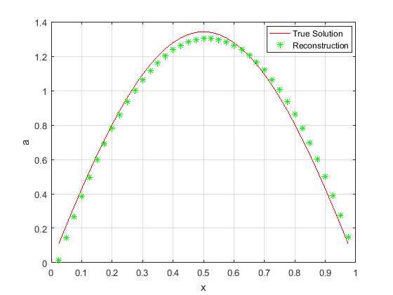
Figure 1. Case(a): True solutions atrue and reconstruction ar
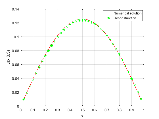
Figure 2. Case(a): Numerical solutions un and reconstruction ur
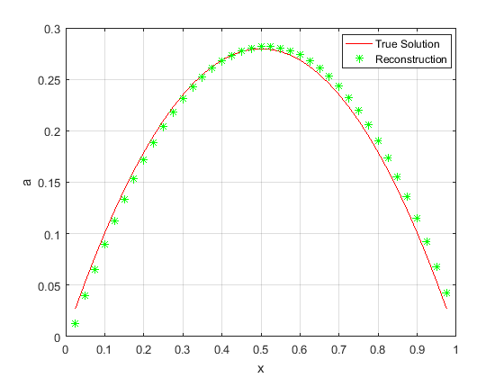
Figure 3. Case(b): True solutions atrue and reconstruction ar
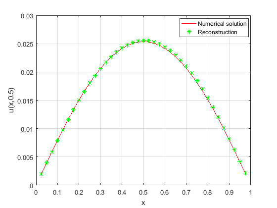
Figure 4. Case(b): Numerical solutions un and reconstruction ur
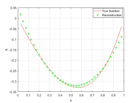
Figure 5. Case(c): True solutions atrue and reconstruction ar
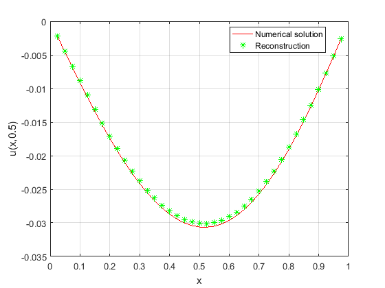
Figure 6. Case(c): Numerical solutions un and reconstruction ur
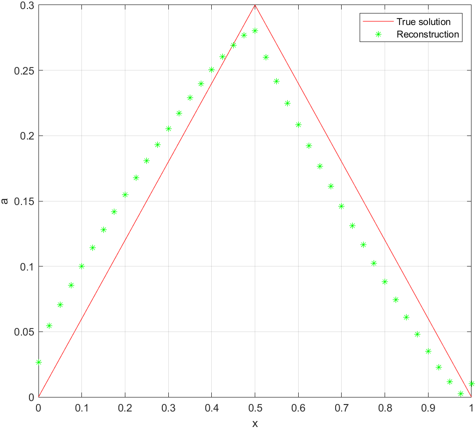
Figure 7. Case(d): True solutions atrue and reconstruction ar
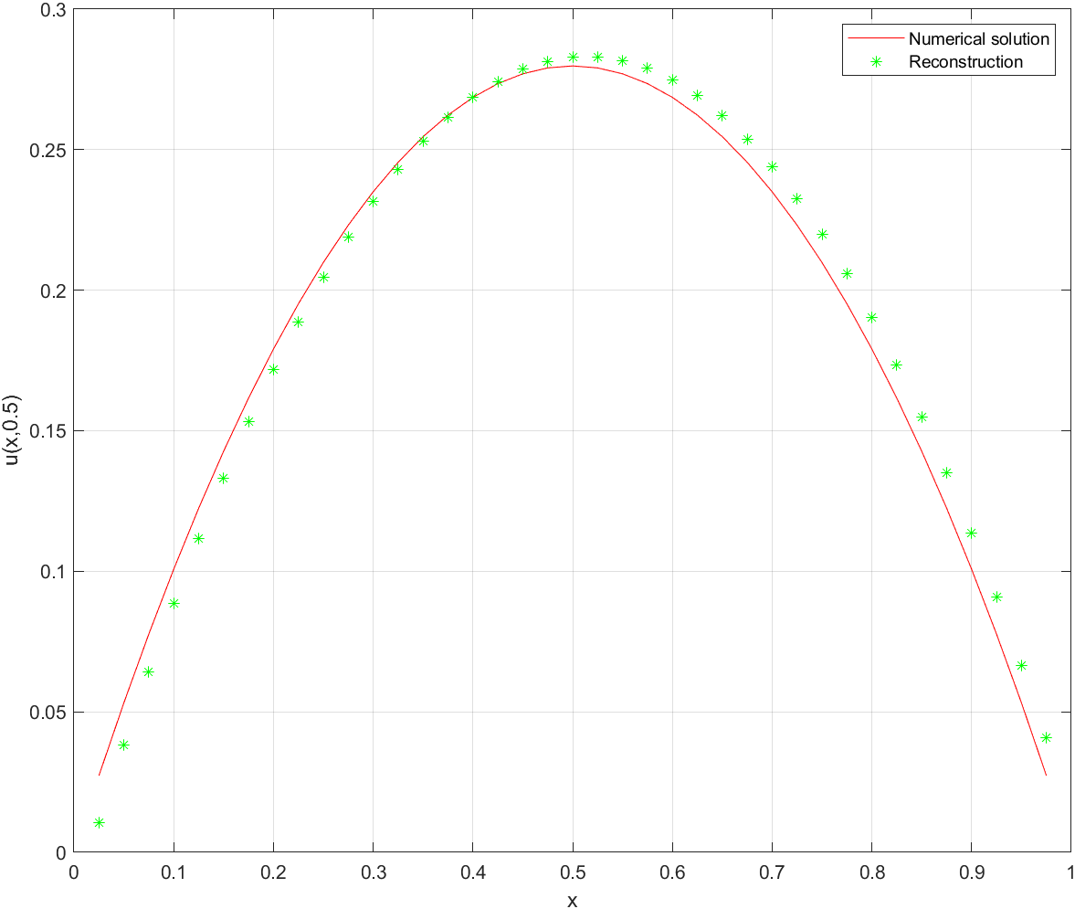
Figure 8. Case(d): Numerical solutions un and reconstruction ur
In figure 1-2, for case(a), the iteration steps \(k=786\) is obtained using the Algorithm (4.1) to obtain the reconstructed solution of the initial value, and the relative error of the reconstructed solution and the true solution of the initial value \(err_{a}=4.71\%\), the relative error of the reconstructed solution of the direct problem obtained by inversion algorithm and the numerical solution obtained by difference scheme \(err_{u}=1.36\%\). In figure 3-4, for case(b), the iteration steps \(k=863\) and the relative error between the reconstructed solution and the true solution of the initial value \(err_{a}=4.36\%\), the relative error of the numerical solution and the reconstructed solution of the direct problem \(err_{u}=1.29\%\). In figure 5-6, for case(c), the iteration steps \(k=1016\) and the relative error between the reconstructed solution and the true solution of the initial value \(err_{a}=6.80\%\), the relative error of the numerical solution and the reconstructed solution of the direct problem \(err_{u}=1.77\%\). In figure 7-8, for case(d), owing to the poor regularity of the target function, the reconstruction results are not as well as those of the smooth case in the previous examples. The iteration steps \(k=2217\) and the relative error between the reconstructed solution and the true solution of the initial value \(err_{a}=12.67\%\), the relative error of the numerical solution and the reconstructed solution of the direct problem \(err_{u}=3.56\%\). Figure 1-6 and the relative error \(err_{a}, err_{u}\) indicate the efficiency and accuracy of the proposed Algorithm (4.1) for simulating the unique continuation.
Concluding remarks
In this paper, on the basis of the Theta function method, we first gave a representation formula of the solution and showed the uniqueness of the solution to the Cauchy problem by the use of the Laplace transform argument, from which we further verified the unique continuation property of the solution to (1.1). Specifically, we proved that a solution to a fractional diffusion equation can be uniquely determined from an interior subdomain. The method used in the proof is new method that can effectively overcome the difficulties caused by the non-locality of fractional derivatives. This result and the used methods not only provide theoretical foundation for the fractional diffusion equations but also open up new possibilities for studying related inverse problems in areas such as inverse source problems and approximate control problem in practical applications.
Let us mention that the proof of the unique continuation principle heavily relies on the Theta function method which enables one to derive an explicit representation formula of the solution. It would be interesting to investigate what happens about the unique continuation property of the solution in the general dimensional case. Moreover, in Theorem 1, we only proved the uniqueness result for determining the solution from the information of the solution in interior domain. In comparison, it is known that conditional stability results hold for the same problems for elliptic or parabolic equations based on Carleman estimates. Unfortunately, such techniques do not work in the case of fractional diffusion equations due to the absence of the fundamental integration by parts for the fractional derivatives.
In the numerical aspect, we reformulate the unique continuation principle as an optimization problem with Tikhonov regularization. After the derivation of the corresponding variational equation, we can characterize the minimizer by employing the associated backward fractional diffusion equation, which results in our iterative method. Then several numerical experiments for the reconstructions are implemented to show the efficiency and accuracy of the proposed Algorithm 4.1 for simulating the unique continuation. Here we point out that the homogeneous boundary condition was assumed in deriving Algorithm 4.1. It will be intriguing to derive Algorithm 4.1 without assuming the homogeneous boundary condition, as the algorithm for the general case still remains a challenge to be solved.
Acknowledgment
This second author was supported by National Natural Science Foundation of China No. 12271277. This work was partly supported by the Open Research Fund of Key Laboratory of Nonlinear Analysis & Applications (Central China Normal University), Ministry of Education, P. R. China.
Conflict of interest:
The authors declare no conflict of interest.
References
Adams, E.E., and Gelhar, L.W. (1992). Field study of dispersion in a heterogeneous aquifer: 2. Spatial moments analysis. Water Resour. Res. 28: 3293–307.View
Cannon, J. (1984). The One-Dimensional Heat Equation, Encyclopedia of Mathematics and Application. Addison-Wesley, Menlo Park, CA, View
Cheng, J., Lin, C-L., and Nakamura, G. (2013). Unique continuation property for the anomalous diffusion and its application. J. Differential Equations, 254: 3715–28.View
Doss, R. (1988). An elementary proof of Titchmarsh¨s convolution theorem. Proceedings of the American Mathematical Society, 104(1): 181–184.View
Fujishiro, K., and Yamamoto, M. (2014). Approximate controllability for fractional diffusion equations by interior control. Appl. Anal. 93(9): 1793–1810.View
Hatano Y, Hatano N. (1998). Dispersive transport of ions in column experiments: An explanation of long-tailed profiles. Water Resources Research, 34(5): 1027–33.View
Jiang, D., Li, Z., Liu, Y. and Yamamoto, M. (2017). Weak unique continuation property and a related inverse source problem for time-fractional diffusion-advection equations. Inverse Problems, 33(5): 055013.View
Eidelman, S.D., Kochubei, A.N. (2004). Cauchy problem for fractional diffusion equations. Journal of Differential Equations, 199(2): 211–255.View
Li, Z., Liu, Y. and Yamamoto, M. (2015). Initial-boundary value problems for multi-term timefractional diffusion equations with positive constant coefficients. Applied Mathematics and Computation, 257: 381–397.View
Li, Z., Yamamoto, M. (2018). Unique continuation principle for the one-dimensional timefractional diffusion equation. Fractional Calculus and Applied Analysis, 22(3): 644–657.View
Lin, C-L., and Nakamura, G. (2016). Unique continuation property for anomalous slow diffusion equation. Commun. Partial Diff. Eqns, 41(5): 749–758.View
Liu Y. (2027). Strong maximum principle for multi-term time-fractional diffusion equations and its application to an inverse source problem. Comput. Math. Appl. 73(1): 96-108.View
Liu, Y., Hu, G. and Yamamoto, M. (2021). Inverse moving source problems for time-fractional evolution equations: determination of profiles. Inverse Probl. 37(8): 084001 (23pp).View
Liu, Y., Rundell, W., Yamamoto, M. (2016). Strong maximum principle for fractional diffusion equations and an application to an inverse source problem. Frac. Calc. Appl. Anal. 19(4): 888–906.View
Luchko Y. (2010). Some uniqueness and existence results for the initial-boundary-value problems for the generalized time-fractional diffusion equation. Comput. Math. Appl. 59(5): 1766–1772..View
Luchko Y. (2011). Initial-boundary-value problems for the generalized multi-term timefractional diffusion equation. J. Math. Anal. Appl. 374(2): 538–48.View
Podlubny I. (1999). Fractional Differential Equations (San Diego: Academic)View
Rundell, W., Xu, X., and Zuo, L. (2013). The determination of an unknown boundary condition in a fractional diffusion equation. Applicable Analysis, 92(7): 1511–1526.View
Sakamoto, K., and Yamamoto, M. (2011). Initial value/boundary value problems for fractional diffusion-wave equations and applications to some inverse problems. J. Math. Anal. Appl. 382: 426–447.View
Sun, C., Liu, J. (2020). Reconstruction of the space-dependent source from partial Neumann data for slow diffusion system. Acta Math. Appl. Engl. Ser. 36: 166–182.View
Titchmarsh, E.C. (1926). The zeros of certain integral functions. Proceedings of the London Mathematical Society, s2-25 (1): 283–302.View
Schiff, J.L. (2013). The Laplace Transform: Theory and Applications. Springer Science & Business Media.View