
- About the Journal
- Editorial Board
- Review Process
- Author Guidelines
- Article Processing Charges
- Special Issues
- Current Issue
- Past Issue
 Journal of Comprehensive Pure and Applied Mathematics
Journal of Comprehensive Pure and Applied Mathematics Volume 2 (2024), Article ID: JCPAM-108
https://doi.org/10.33790/cpam1100108Research Article
The Topology of Subspaces of the Configuration Space of Spatial Hexagons
Yasuhiko Kamiyama
*Department of Mathematics, University of the Ryukyus, Nishihara- Cho, Okinawa 903-0213, Japan.
Corresponding Author Details: Department of Mathematics, University of the Ryukyus, Nishihara- Cho, Okinawa 903-0213, Japan.
Received date: 19th March, 2024
Accepted date: 24th April, 2024
Published date: 27th April, 2024
Citation: Kamiyama, Y. (2024).The Topology of Subspaces of the Configuration Space of Spatial Hexagons. J Comp Pure Appl Math, 2(1): 108.
Copyright: ©2024, This is an open-access article distributed under the terms of the Creative Commons Attribution License, which permits unrestricted use, distribution, and reproduction in any medium, provided the original author and source are credited.
Abstract
We assume that four bond angles of a spatial hexagon are \(\theta\). According to the choice of the four bond angles, we define the configuration spaces \(X_6(\theta)\), \(Y_6(\theta)\) and \(Z_6(\theta)\). We determine the topological types of these spaces.
Introduction
In [6], we determined the topological type of the configuration space of spatial pentagons whose two bond angles are \(\theta\). In this paper, we determine the topological type of the configuration space of spatial hexagons whose four bond angles are \(\theta\).
Let \(M_n\) be the configuration space of equilateral polygons in \({\mathbb R}^3\). The seminal paper [7] studied \(M_n\) from the viewpoint of symplectic geometry. After this, many mathematicians studied various aspects of \(M_n\). We refer to [2] for an excellent exposition with emphasis on Morse theory.
Recently, mathematicians and chemists are interested in the mathematical models for chemical compounds. (See, for example, [1, 4, 8]) For some cases, their configuration spaces are subspaces of \(M_n\). The rule which connects mathematics and chemistry is the following:
Rule 1. Recall that a monocyclic hydrocarbon consists of single bonds and double bonds. We impose the following rules. We fix \(\theta \in (0,\pi)\).
(i) The bond angle formed by adjacent single bonds are \(\theta\).
(ii) The bond angles of the both ends of a double bond are arbitrary.
Hereafter we consider a monocyclic hydrocarbon which have \(6\)-bonds.
Example 2. Among monocyclic hydrocarbons, the benzene is most famous. The benzene is defined as the left-end of Figure 1. By Rule 1 (ii), all bond angles of a hexagon are arbitrary. Hence the space of benzenes can be identified with \(M_6\).
Example 3. The cyclohexane is defined as the middle of Figure 1. By Rule 1 (i), the set of cyclohexanes can be identified with the configuration space of equilateral and equiangular hexagon. Recall that [8] obtained a complete information on the configuration space of these hexagons.
Example 4. The cyclohexene is defined as the right-end of Figure 1. By Rule 1 (i) and (ii), the space of cyclohexenes can be identified with the configuration space of the equilateral hexagons whose first four bond angles are \(\theta\). (See \(X_6(\theta)\) in Definition 5 (i).)
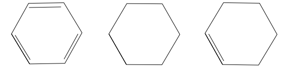
Figure: 1 Left: Benzene. Middle: Cyclohexane. Right: Cyclohexene.
If we forget chemical backgrounds, we have some more ways to impose conditions on the bond angles of a polygon. In this case, we may regard a polygon as a mechanical linkage. As an example, we consider the following two more subspaces of \(M_6\).
Definition 5. We fix \(\theta\in (0,\pi)\) and define the spaces \(X_6(\theta)\), \(Y_6(\theta)\) and \(Z_6(\theta)\) as follows.
(i) We set \[\begin{aligned} X_6(\theta):=\{(v_1,\dots,v_6) \in ({\mathbb R}^3)^6 \,\;\vert\,\;&\text{the following conditions (a), (b)}\\ &\qquad \text{and (c) hold}\}. \end{aligned}\] Here
(a) \(v_1=(0,0,0)\), \(v_2=(1,0,0)\) and \(v_3=(1-\cos \theta,\sin \theta,0)\).
(b) \(\Vert v_{i+1}-v_i \Vert=1\) for \(2 \leq i \leq 5\) and \(\Vert v_1-v_6\Vert=1\).
(c) \(\angle v_iv_{i+1} v_{i+2}=\theta\) for \(2\leq i \leq 4\).
(See the left-end of Figure 2
(ii) We set \[\begin{aligned} Y_6(\theta):=\{(v_1,\dots,v_6) \in ({\mathbb R}^3)^6 \,\;\vert\,\;&\text{the above conditions (a), (b)}\\ & \text{and the following condition (d) hold}\}. \end{aligned}\] Here
(d) \(\angle v_iv_{i+1}v_{i+2} =\theta\) for \(2\leq i \leq 3\) and \(\angle v_5v_6 v_1=\theta\).
(See the middle of Figure 2.)
(iii) We set \[\begin{aligned} Z_6(\theta):=\{(v_1,\dots,v_6) \in ({\mathbb R}^3)^6 \,\;\vert\,\;&\text{the above conditions (a), (b)}\\ &\text{and the following condition (e) hold}\}. \end{aligned}\] Here
(e) \(\angle v_iv_{i+1}v_{i+2} =\theta\) for \(i\in \{2,4\}\) and \(\angle v_5v_6 v_1=\theta\).
(See the right-end of Figure 2.)
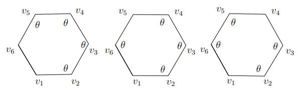
Figure: 2 Left: An element of\(X_6(\theta)\). Middle: An element of \(y_6(\theta)\). Right: An element of \(z_6(\theta)\).
Remark 6. (i) The space \(X_6(\theta)\) is the mathematical formulation of the space which is considered in Example 4.
(ii) The spaces \(X_6(\theta)\), \(Y_6(\theta)\) and \(Z_6(\theta)\) are defined by requiring that certain four bond angles of a hexagon are \(\theta\). In fact, if we require that four bond angles of a hexagon are \(\theta\), then the space we obtain is \(X_6(\theta)\), \(Y_6(\theta)\) or \(Z_6(\theta)\).
The purpose of this paper is to determine the topological types of \(X_6(\theta)\), \(Y_6(\theta)\) and \(Z_6(\theta)\). This paper is organized as follows. In §2 we state our main results. The topological types of \(X_6(\theta)\), \(Y_6(\theta)\) and \(Z_6(\theta)\) are determined in Theorems A, B and C, respectively. In §3 we apply Morse theory to a robot arm, which is used in later sections. We prove Theorems A, B and C in §4, 5 and 6, respectively. In §7 we give conclusions.
Main Results
Theorem A . The topological type of \(X_6(\theta)\) is given by the following Table 1, where following to the Schläfli symbol, \(\{6\}\) denotes the regular hexagon.
\[\begin{array}{|c|c|c|c|c|c|}\hline \theta & (0,\frac{\pi}{3}) & (\frac{\pi}{3},\frac{\pi}{2}) & (\frac{\pi}{2},\frac{2}{3}\pi) & \frac{2}{3}\pi & (\frac{2}{3}\pi,\pi) \\ \hline \text{Topological type} & \underset{3}{\#}(S^1 \times S^1) & \underset{3}{\#}(S^1 \times S^1) & S^2 & \{ 6\} & \varnothing \\ \hline \end{array}\]
Remark 7. The topological types of \(X_6(\frac{\pi}{3})\) and \(X_6(\frac{\pi}{2})\) are determined in [4].. In particular, they have singular points.
Theorem B . The topological type of \(Y_6(\theta)\) is given by the following Table 2
\[\begin{array}{|c|c|c|c|c|c|}\hline \theta & (0,\frac{\pi}{3}) &\frac{\pi}{3}& (\frac{\pi}{3},\frac{2}{3}\pi)& \frac{2}{3}\pi & (\frac{2}{3}\pi,\pi)\\ \hline \text{Topological type} & (S^1 \times S^1) \amalg (S^1 \times S^1) & S^1 \times U & S^1 \times S^1 & S^1 & \varnothing\\ \hline \end{array}\]
Here we define \(U\) as the left of Figure 3.
Theorem C. The topological type of \(Z_6(\theta)\) is given by the following Table 2.
\[\begin{array}{|c|c|c|}\hline \theta & (0,\frac{\pi}{3}) &(\frac{\pi}{3},\pi)\\ \hline \text{Topological type} & S^1 \times V & S^1 \times V\\ \hline \end{array}\]
Here we define \(V\) as the right of Figure 3.
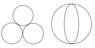
Figure: 3 Left: U. Right: V .
Remark 8. The space \(Z_6(\frac{\pi}{3})\) has a complicated singularity. See §7 for more details.
Morse theory of a robot arm
We define \[M_n(\theta):= \left\{(a_1,\dots,a_n)\in (S^2)^n\,\;\vert\,\;\text{the following conditions (I) and (II) hold}\right\}.\] Here
(I) \(a_1=(1,0,0) \; \text{and}\; a_2=(-\cos \theta,\sin \theta,0).\)
(II) \(\langle a_i,a_{i+1}\rangle =-\cos \theta \; (1 \leq i \leq n-1),\) where \(\langle,\rangle\) denotes the standard inner product on \({\mathbb R}^3\).
We also define \[\begin{aligned} \label{oct12c} N_{n+1}(\theta):=\{(v_1,\dots,v_{n+1}) \in ({\mathbb R}^3)^{n+1} \,\;\vert\,\;& \text{the following conditions (III)}\\ &\text{(IV) and (V) hold}\}.\notag \end{aligned}\]
Here
(III) \(v_1=(0,0,0)\), \(v_2=(1,0,0)\) and \(v_3=(1-\cos \theta,\sin \theta,0)\).
(IV) \(\Vert v_{i+1}-v_i \Vert=1\) for \(1 \leq i \leq n\).
(V) \(\angle v_iv_{i+1} v_{i+2}=\theta\) for \(1\leq i \leq n-1\).
Lemma 9. We have the following homeomorphisms \(\alpha\) and \(\beta\): \[\label{albe} \begin{CD} (S^1)^{n-2} @>\alpha>\cong> M_n(\theta) @>\beta>\cong > N_{n+1}(\theta). \end{CD}----(2)\]
Proof. First, we construct \(\alpha\). From an element \[(e^{i \phi_1},\cdots,e^{i \phi_{n-2}})\in (S^1)^{n-2},\] we construct the element \((a_1,\cdots,a_n)\in M_n(\theta)\) as follows: In the process of constructing \(a_i\), we also construct the elements \(n_i \in S^2\) such that \(\langle a_i,n_i\rangle=0\). We set \[\begin{aligned} a_{i+2}:=&\, -(\cos \theta) a_{i+1}+(\sin\theta \cos \phi_i )n_{i+1}+(\sin \theta \sin \phi_i) a_{i+1}\times n_{i+1}----(3) \label{ga}\\ and n_{i+2}:=&\, -(\sin \theta) a_{i+1}-(\cos\theta \cos \phi_i )n_{i+1}-(\cos \theta \sin \phi_i) a_{i+1} \times n_{i+1},----(4)\label{de} \end{aligned}\] where \(a_{i+1}\times n_{i+1}\) denotes the cross product.
We set \[\begin{aligned} &a_1=(1,0,0),\quad n_1=(0,1,0)\\ &a_2= (-\cos \theta, \sin \theta,0)\quad \text{and}\quad n_2=(-\sin \theta,-\cos \theta,0). \end{aligned}\] From 3 and 4 for \(i=1\), we obtain \(a_3\) and \(n_3\). Next from 3 and 4 for \(i=2\), we obtain \(a_4\) and \(n_4\). Repeating this process, we obtain \(a_i\) and \(n_i\) for \(1 \leq i \leq n\). Now we define \(T\) by \[\alpha(e^{i \phi_1},\cdots,e^{i \phi_{n-2}})=(a_1,\cdots,a_n).\] From the construction, \(\alpha\) is a diffeomorphism.
Second, we construct \(\beta\). For \((a_1,\dots,a_n)\in M_n(\theta)\), we set \[v_i:= \begin{cases} (0,0,0),&\quad \text{if $i=1$,}\\ \displaystyle{\sum_{q=1}^{i-1}a_q} ,& \quad \text{if $2\leq i \leq n+1$.} \end{cases}\] It is clear that \((v_1,\dots,v_{n+1})\in N_{n+1}(\theta)\). We define \(\beta\) by \[\label{summ} \beta(a_1,\dots,a_n)=(v_1,\dots,v_{n+1}).----(5)\] Then from 5, \(\beta\) is a homeomorphism. ◻
Definition 10. (i) We define the homeomorphism \[T:(S^1)^{n-2}\to N_{n+1}(\theta)\] by \(T:=\beta \circ \alpha.\)
(ii) We define the function \[f_{n+1,\theta}: N_{n+1}(\theta) \to {\mathbb R}\] by \[f_{n+1,\theta}(v_1,\dots, v_{n+1}):=\Vert v_{n+1}\Vert.\]
Note that \[\label{oct10b} f_{6,\theta}^{-1}(1)=X_6(\theta).----(6)\]
The following Lemmas 11 and 12 are keys to proving Theorem A.
Lemma 11 (i) We define the function \[\label{nov15a} g:(S^1)^3\times (0,\pi)\to {\mathbb R}----(7)\] by \[g(e^{i\phi_1},e^{i\phi_2},e^{i\phi_3},\theta)=(f_{6,\theta}\circ T) (e^{i\phi_1},e^{i\phi_2},e^{i\phi_3})-1.\] Then \(g^{-1}(0)\) is a manifold.
(ii) We define the function \(h: (S^1)^3 \times (0,\pi)\to {\mathbb R}\) by \[h(e^{i\phi_1},e^{i\phi_2},e^{i\phi_3},\theta)=\theta.\] Let \(\bar{h}\) be the restriction of \(h\) to \({g^{-1}(0)}\): \(\bar{h}:= \left. h\right|_{g^{-1}(0)}.\) Then the critical points of \(\bar{h}\) are given by the following Table 4, , where ‘‘number" means the number of critical points.
| \(\text{critical value}\) | \(\text{number}\) | \(\text{index}\) | \(\text{degeneracy}\) |
|---|---|---|---|
| \(\frac{2}{3}\pi\) | \(1\) | \(3\) | \(\text{non-degenerate}\) |
| \(\frac{\pi}{2}\) | \(3\) | \(2\) | \(\text{non-degenerate}\) |
| \(\frac{\pi}{3}\) | \(\infty\) | \(\text{degenerate}\) |
Proof. In [4], similar assertions are proved in detail. The key of the proofs are as follows.
(i) Using the implicit function theorem, we obtain (i).
(ii) We need to determine maximal elements and minimal elements the critical point of \(h\) under the restriction \(g=0\). Then using the method of Lagrange multiplier, we obtain (ii). ◻
Using Table 4, we can determine the topological type of \(X_6(\theta)\) for \(\frac{\pi}{3}<\theta<\pi\). (See §4 for more details.) On the other hand for the case \(0<\theta<\frac{\pi}{3}\), we need the following information.
Lemma 12. Assume that \(0<\theta<\frac{\pi}{3}\). Then we have the following:
(i) The critical points of \(f_{6,\theta}\) are given by the following Table 5.
| \(\text{critical value}\) | \(\text{number}\) | \(\text{index}\) | \(\text{degeneracy}\) |
|---|---|---|---|
| \(\sqrt{13-12\cos \theta}\) | \(1\) | \(3\) | \(\text{non-degenerate}\) |
| \(3-2\cos \theta\) | \(1\) | \(2\) | \(\text{non-degenerate}\) |
| \(\sqrt{7-10\cos \theta+6\cos 2\theta-2\cos 3\theta}\) | \(2\) | \(2\) | \(\text{non-degenerate}\) |
| \(\sqrt{9-12\cos \theta+4\cos 2\theta}\) | \(3\) | \(1\) | \(\text{non-degenerate}\) |
| \(1-2\cos \theta+2\cos 2\theta\) | \(1\) | \(0\) | \(\text{non-degenerate}\) |
(ii) Let \(\xi\) be a critical value in Table 5. Then we have \(\xi>1\) if and only if \(\xi\) is either \[\sqrt{13-12\cos \theta},\; 3-2\cos \theta \;\; \text{or}\;\; \sqrt{7-10\cos \theta+6\cos 2\theta-2\cos 3\theta}.\]
Proof. (i) Since we can write \(f_{6,\theta}\circ T\) explicitly, we obtain the lemma from direct computations.
(ii) Using the fact that \(0<\theta<\frac{\pi}{3}\), it is easy to prove the item. ◻
The following Proposition 13 is a key to proving Theorem B.
Proposition 13. The topological type of \(f_{5,\theta}^{-1} (2\sin \frac{\theta}{2})\) is given by the following Table 6.
\[\begin{array}{|c|c|c|c|c|c|}\hline \theta & (0,\frac{\pi}{3}) &\frac{\pi}{3}& (\frac{\pi}{3},\frac{2}{3}\pi)& \frac{2}{3}\pi & (\frac{2}{3}\pi,\pi)\\ \hline \text{Topological type} & S^1 \amalg S^1 & U & S^1 & \text{one point} & \varnothing\\ \hline \end{array}\] Table 6. The topological type of \(f_{5,\theta}^{-1} (2\sin \frac{\theta}{2})\)
In order to prove Proposition 13, we prove the following Lemmas 14 and 15.
Lemma 14. (i) We define the function \[g_1:(S^1)^2\times (0,\pi)\to {\mathbb R}----(8)\] by \[g_1(e^{i\phi_1},e^{i\phi_2},\theta)=(f_{5,\theta}\circ T) (e^{i\phi_1},e^{i\phi_2})-2\sin\frac{\theta}{2}.\] Then \(g_1^{-1}(0)\) is a manifold.
(ii) We define the function \(h_1: (S^1)^2 \times (0,\pi)\to {\mathbb R}\) by \[h_1(e^{i\phi_1},e^{i\phi_2},\theta)=\theta.\] Let \(\bar{h}_1\) be the restriction of \(h_1\) to \({g_1^{-1}(0)}\): \(\bar{h}_1:= \left. h_1\right|_{g_1^{-1}(0)}.\) Then the critical points of \(\bar{h}_1\) are given by the following Table 7.
| \(\text{critical value}\) | \(\text{number}\) | \(\text{index}\) | \(\text{degeneracy}\) |
|---|---|---|---|
| \(\frac{2}{3}\pi\) | \(1\) | \(2\) | \(\text{non-degenerate}\) |
| \(\frac{\pi}{3}\) | \(3\) | \(1\) | \(\text{non-degenerate}\) |
Proof. We can prove the lemma in the same way as in Lemma 11. ◻
Similarly to Table 5, we also need the following:
Lemma 15. Assume that \(0<\theta<\frac{\pi}{3}\). Then the critical points of \(f_{5,\theta}\) are given by the following Table 6.
| \(\text{critical value}\) | \(\text{number}\) | \(\text{index}\) | \(\text{degeneracy}\) |
|---|---|---|---|
| \(4\sin \frac{\theta}{2}\) | \(1\) | \(\text{degenerate}\) | |
| \(4\cos \theta \sin \frac{\theta}{2}\) | \(1\) | \(1\) | \(\text{non-degenerate}\) |
| \(4 \sin^2 \frac{\theta}{2}\) | \(2\) | \(1\) | \(\text{non-degenerate}\) |
| \(0\) | \(2\) | \(0\) | \(\text{non-degenerate}\) |
Proof. By computing \(f_{5,\theta}\circ T\), we can prove the lemma in the same way as in Lemma 12. ◻
Proof of Proposition 13 Note that we have the homeomorphism \[\left. T\right|_{{h}_1^{-1}(\theta)}: {h}_1^{-1}(\theta)\to f_{5,\theta}^{-1} (2\sin \frac{\theta}{2}).\]
(i) The case \(\frac{\pi}{3}<\theta\leq \pi\). By Table 7, we have \(\max \bar{h}=\frac{2}{3}\pi\). Hence Table 6 is true for \(\frac{2}{3}\pi \leq \theta\leq \pi\). Moreover, applying the Morse lemma to Table 7, we see that Table 6 is true for \(\frac{\pi}{3}<\theta< \frac{2}{3}\pi\).
(ii) The case \(0<\theta<\frac{\pi}{3}\). Note that in Table 8, we have \[4 \sin^2 \frac{\theta}{2}<2\sin \frac{\theta}{2}<4\cos \theta\sin \frac{\theta}{2}.\] We set \[H:= f_{5,\theta}^{-1} [2\sin \frac{\theta}{2},4\sin \frac{\theta}{2} ].\] Note that \[\label{oct11c} f_{5,\theta}^{-1} (2\sin \frac{\theta}{2})=\partial H.----9\] We study the handle decomposition of \(H\).
In Table 8, the critical point which gives the global maximum is degenerate. Nevertheless, using [3, Lemma 1], there is a diffeomorphism \[\label{oct11a} f_{5,\theta}^{-1}[\xi, 4\sin \frac{\theta}{2} ]\cong D^2,----10\] for all \(\xi \in (4\cos \theta\sin \frac{\theta}{2},4\sin \frac{\theta}{2})\).
Using (10) and Table 8, \(H\) has a form \[\label{oct11b} H= D^2 \cup (D^1\times D^1).----11\] That is, \(H\) is a Möbius strip or an annulus. Below we show that \(H\) is in fact an annulus: Note that \(H\) is a subspace of \(N_5(\theta)\). Moreover, \(N_5(\theta)\) is homeomorphic to \((S^1)^2\) by Lemma 9. Hence (11) in fact implies that\[\label{mar21} H=S^1 \times D^1.----12\]
Now we have from (12) that \(\partial H=S^1 \amalg S^1.\) Then using (9), we have \[f_{5,\theta}^{-1} (2\sin \frac{\theta}{2})=S^1 \amalg S^1.\]
(iii) The case \(\theta=\frac{\pi}{3}\). Note that in this case, we have \(2\sin \frac{\theta}{2}=1\). Consider the equation \[\label{oct11f} f_{5,\theta}\circ T (e^{i\phi_1},e^{i\phi_2})=1,----(13)\] with variables in \(\phi_1\in [0,2\pi]\) and \(\phi_2 \in [-\pi,\pi]\).
We define \(C_1\), \(C_2\) and \(C_3\) as follows. \[\begin{aligned} C_1=& \{(\phi_1,\phi_2) \in [0,2\pi]\times [-\pi,\pi]\,\;\vert\,\;\phi_2=-2 \arctan \left(2\cot \frac{x}{2}\right)\},\\ C_2=& \{(\phi_1,\phi_2) \in [0,2\pi]\times [-\pi,\pi]\,\;\vert\,\;\phi_1=0\}\\ {and} C_3=& \{(\phi_1,\phi_2) \in [0,2\pi]\times [-\pi,\pi]\,\;\vert\,\;\phi_2=0\}: \end{aligned}\] It is easy to see that the complete solution of (13) is given by \(C_1\cup C_2 \cup C_3\). Now since the figure of \(C_1\cup C_2 \cup C_3\) is homeomorphic to \(U\), Proposition 13 holds for \(\theta=\frac{\pi}{3}\). ◻
Proof of Theorem A
Proof of Theorem A. (i) The case for \(\frac{\pi}{2}< \theta<\pi\). The case is clear from Table 4.
(ii) The case for \(\frac{\pi}{3}<\theta<\frac{\pi}{2}\). Table 4 tells us that \(X_6(\theta)\) is obtained from \(S^2\) by attaching three handles. Equivalently, \(X_6(\theta)=\underset{3}{\#}(S^1 \times S^1).\)
(iii) The case for \(0<\theta<\frac{\pi}{3}.\) In Table 5, there is only one critical point whose index is 3. Hence \(X_6(\theta)\) is connected. Then using Table 5 and Lemma 12 (ii), \(X_6(\theta)\) is obtained from \(S^2\) by attaching three handles. Equivalently, \(X_6(\theta)=\underset{3}{\#}(S^1 \times S^1).\) ◻
Remark 16. The above proof was outlined in [5,6].
Proof of Theorem B
Lemma 17. We have the following homeomorphism \[Y_6(\theta)\cong S^1 \times f_{5,\theta}^{-1} (2\sin \frac{\theta}{2}).\]
Proof. We define the \(S^1\)-action on \(Y_6(\theta)\) as follows: For \((v_1,\dots,v_6)\in Y_6(\theta)\), let \(v_6\) rotate about the diagonal \(v_1v_5\).
Since \[\Vert v_1-v_5\Vert =2 \sin \frac{\theta}{2},\] we have \[Y_6(\theta)/S^1= f_{6,\theta}^{-1} (2\sin \frac{\theta}{2}).\] Hence there is a principal bundle \[S^1 \to Y_6(\theta) \to f_{5,\theta}^{-1} (2\sin \frac{\theta}{2}).\] Since \(f_{5,\theta}^{-1} (2\sin \frac{\theta}{2})\) is a one-dimensional space, the bundle is trivial.◻
Proof of Theorem B. Combining Lemma 17 and Corollary 13, we obtain Theorem B.◻
Proof of Theorem C
Lemma 18. Let \(P\) be the fiber product of the following diagram: \[\label{fib} \begin{CD} P @>>> N_4(\theta)\\ @VVV @VV f_{4,\theta}V\\ N_4(\theta) @> f_{4,\theta} >> {\mathbb R} \end{CD}----(14)\] Then there is a homeomorphism \[Z_6(\theta)\cong S^1 \times P.\]
Proof. We define the \(S^1\)-action on \(Z_6(\theta)\) as follows: The \(S^1\) rotate the quadrilateral \(v_1v_4v_5v_6\) about the diagonal \(v_1v_4\). Then there is a principal bundle \[\label{oct12e} S^1 \to Z_6(\theta) \to Z_6(\theta)/S^1.----(15)\] Since \(Z_6(\theta)/S^1\) is a one-dimensional space, (15) gives a homeomorphism \[\label{oct12f} Z_6(\theta) \cong S^1 \times Z_6(\theta)/S^1.----(16)\]
Lemma 19. We assume that \(\theta \not= \frac{\pi}{3}\). Then there is a homeomorphism \[\label{oct12g} \Phi: P \to Z_6(\theta)/S^1.\]
Proof of Lemma 19. We use \(v_1\), \(v_2\) and \(v_3\) as in Definition 5(i)(a). Take an element \[((v_1,v_2,v_3,w_4),(v_1,v_2,v_3,v_4))\in P.\] This element is illustrated as the left-end and middle figures of the following Figure 4. Let \(\zeta\) be an orientation-preserving isometry which satisfies the following conditions: \[\label{nov13} \zeta(w_4)=v_1 \;\; \text{and}\;\; \zeta(v_1)=v_4.----(17)\] Then we define \(\Phi\) by \[\label{r} \Phi((v_1,v_2,v_3,w_4),(v_1,v_2,v_3,v_4))=(v_1,v_2,v_3,v_4, \zeta(v_2),\zeta(v_3)).----(18)\] Here the right-hand side of (18) is illustrated as the right-end figure of the following Figure 4.
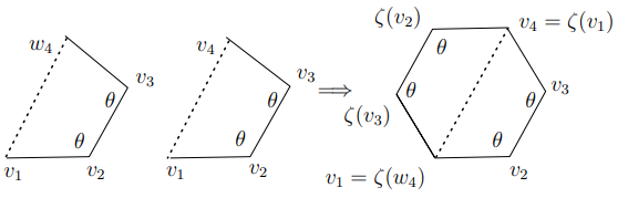
Figure: 4 The homeomorphism \(\Phi\): P\(Z_6(\theta)/S^1\).
Although the freedom of the choice of \(\zeta\) is \(S^1\), the map \(\Phi\) in (18) is well-defined as a map to \(Z_6(\theta)/S^1\). We shall prove that \(\Phi\) is a homeomorphism.
Surjectivity: Since we are assuming \(\theta \not= \frac{\pi}{3}\), it is clear that \(\Phi\) is surjective. (See §7 for the case \(\theta=\frac{\pi}{3}\).)
Injectivity: Assume that two elements of \(P\) satisfy \[\label{iso1} \Phi((v_1,v_2,v_3,w_4),(v_1,v_2,v_3,v_4))=\Phi((v_1,v_2,v_3,W_4),(v_1,v_2,v_3,V_4)).----(19)\]
First, it is clear from (18) that \[\label{v1} v_4=V_4.----(20)\]
Second, choosing orientation-preserving isometries \(\zeta\) and \(\eta\), we construct quadrilaterals \(\zeta (v_1) \zeta(v_2) \zeta (v_3) \zeta(w_4)\) and \(\eta(v_1) \eta(v_2) \eta(v_3)\eta (W_4)\), where we choose \(\zeta\) and \(\eta\) so as to satisfy the following conditions (see 17: \[\label{oct27c} \zeta(v_1)=\eta(v_1)=v_4, \;\; \text{and} \;\;\zeta(w_4)=\eta(W_4)=v_1.----(21)\] Then (19) implies that these quadrilaterals overlap under a rotation about the common side \(v_1v_4\), where we have \(v_4=V_4\) by (20). More precisely, there exists an orientation-preserving isometry \(\rho\) which satisfies the following conditions: \[\begin{aligned} \rho(v_1)=v_1\;\; &\text{and}\;\; \rho(v_4)=v_4 ----(22)\label{ga1}\\ {and} \rho (\zeta (v_2))=\eta(v_2)\;\;&\text{and}\;\; \rho(\zeta(v_3))= \eta(v_3). ----(23)\label{ga2} \end{aligned}\] From (21), (22) and (23) we have \[(\rho \circ \zeta) (v_2-v_1)=\eta (v_2-v_1) \;\; \text{and}\;\; (\rho \circ \zeta) (v_3-v_2)=\eta (v_3-v_2).\] Since \(v_2-v_1\) and \(v_3-v_2\) are linearly independent vectors, we have \[\rho \circ \zeta=\eta.\] Then using (21) and (22), we have
\[\eta(w_4)=(\rho \circ \zeta)(w_4)=v_1=\eta(W_4).\] Hence we obtain \(w_4=W_4\). This completes the proof of the fact that \(\Phi\) is injective.
Now we have proved that \(\Phi\) in (18) is a homeomorphism. Hence the proof of Lemma 19 completes. ◻
Now combining (16) and Lemma 19, we complete the proof of Lemma 18. ◻
Lemma 20. There is a homeomorphism \[P\cong V,\] where \(V\) is defined in Figure 3.
Proof. It is easy to see that \[\label{oct14y} (f_{4,\theta}\circ T)(e^{i\phi_1})=c_1+c_2\cos \phi_1----(24)\] for some \(c_1>0\) and \(c_2<0\). Let \(\mu:S^1 \to {\mathbb R}\) be the height function. Then (24) tells us that \(f_{4,\theta}\) is essentially the same as \(\mu\). Hence we may redefine \(P\) in Lemma 18 as the fiber product of the following diagram: \[\label{redef} \begin{CD} P @>>> S^1\\ @VVV @VV \mu V\\ S^1 @> \mu >> {\mathbb R} \end{CD}\] Then we can write \(P\) as follows. \[\label{oct144} P=\{(\xi,\xi)\,\;\vert\,\;\xi \in S^1\} \cup \{(\xi,\tau(\xi))\,\;\vert\,\;\xi \in S^1\},----(25)\] where for \(\xi=(x_1,x_2)\), we set \(\tau(\xi):= (-x_1,x_2)\). Since the right-hand side of (25) is homeomorphic to \(V\), Lemma 20 holds. ◻
Proof of Theorem C. The theorem follows from Lemmas 18 and 20. ◻
conclusions
Theorem C does not hold for the case \(\theta=\frac{\pi}{3}\). The reason is that \(\Phi\) in Lemma 19 is not surjective. In fact, we set \[W:=\left\{(v_1,\dots,v_6)\in Z_6\left(\frac{\pi}{3}\right)\,\;\vert\,\;v_4=v_1\right\}.\] Then \(W\) is not in the image of \(\Phi\). Note that we have a homeomorphism \(W \cong SO(3)\). Then we pose the following:
Question 21. Does the following homotopy equivalence hold? \[Z_6\left(\frac{\pi}{3}\right)\simeq (S^1\times V) \vee SO(3).\]
Acknowledgments
The author is grateful to the reviewers for many useful comments.
Conflict of Interests:
The author declares that there is no conflicts of interest.
References
Crippen, G. M. (1992). Exploring the conformation space of cycloalkanes by linearized embedding, J. Comput. Chem. 13, 351-361.View
Farber, M. (2008). Invitation to Topological Robotics, Zurich Lectures in Advanced Mathematics, European Mathematical Society (EMS).View
Kamiyama, Y. (2015). On the level set of a function with degenerate minimum point, Int. J. Math. Math. Sci, Art. ID 493217.View
Kamiyama, Y. (2022). The topology of the configuration space of a mathematical model for cycloalkenes, Advanced Topics of Topology, IntechOpen, London. View
Y. Kamiyama, Y. (2023). On the Morse property for the distance function of a robot arm, Motion Planning for Dynamic Agents, IntechOpen, London. https: //www.intechopen.com/chapters/1169815View
Kamiyama, Y. (2023). The topology of subspaces of the configuration space of spatial pentagons, JP J. Geom. Topol. 29, 173-185.View
Kapovich, M., and Millson, J. (1996). The symplectic geometry of polygons in Euclidean space, J. Differential Geom. 44, 479-513.View
O'Hara, J. (2013). The configuration space of equilateral and equiangular hexagons, Osaka J. Math. 50, 477-489. View