
- About the Journal
- Editorial Board
- Review Process
- Author Guidelines
- Article Processing Charges
- Special Issues
- Current Issue
- Past Issue
 Journal of Comprehensive Pure and Applied Mathematics
Journal of Comprehensive Pure and Applied Mathematics Volume 3 (2025), Article ID: JCPAM-115
https://doi.org/10.33790/jcpam1100115Research Article
Exploring Phase-Lock Equations as Nonlinear Ordinary Differential Equations
Mohammad Mahbubur Rahman, Kening Wang*, Mei-Qin Zhan
Department of Mathematics and Statistics, University of North Florida, Jacksonville, FL 32224, USA.
Corresponding Author Details: Kening Wang, Department of Mathematics and Statistics University of North Florida, Jacksonville, FL 32224, USA.
Received date: 13th November, 2024
Accepted date: 08th January, 2025
Published date: 11th January, 2025
Citation: Rahman, M.M., Wang, K., and Zhan, M-Q. (2025). Exploring Phase-Lock Equations as Nonlinear Ordinary Differential Equations. J Comp Pure Appl Math, 3(1):1- 18.
Copyright: ©2025, This is an open-access article distributed under the terms of the Creative Commons Attribution License 4.0, which permits unrestricted use, distribution, and reproduction in any medium, provided the original author and source are credited.
Abstract
In this paper, we derive a simplified version of the phase-lock equations (PLE) that arises in the study of Ginzburg-Landau equations of superconductivity. Our goal is to diffuse the results to an audience who is not entirely familiar with theoretical dynamic behavior, existence, uniqueness, and continuation of solutions of partial differential equations (PDE) on abstract space, but might nonetheless be interested in the practical simulation and connections of dynamical systems versus the numerical issues of PDE in a simpler space. The significant features observed in PLE are their strong attracting sets and basin of attractions resident in the PLE system, which may be beneficial to physicists and engineers in the context of superconductivity. We also explore numerically and graphically the sensitivity of PLE solutions with a variety of forcing functions and parameters.
Introduction
It is well known that time-dependent Ginzburg-Landau equations have been widely used to analyze superconductivity phenomena with an applied electromagnetic field both theoretically and numerically [1, 3, 8]. The existence of time-periodic solutions to Ginzburg-Landau equations has been investigated by many researchers. In 1999, Wang proved the existence of at least one time-periodic solution to the Ginzburg-Landau equations with \(d = 2\) [4], and in 2000, Zhan extended the result to the case with \(d = 3\) [9]. However, because of the higher-order expansion terms of the order parameter, such equations are nonlinear, making the theoretical analysis very limited and complicated. In 2000, Zhan [9] studied the connections between phased-lock equations and time-dependent Ginzburg-Landau equations, and pointed out that these two equations are closely related with certain transformations. Phase-lock equations describe the mathematical relationship within a phase-locked loop system. Compared with time-dependent Ginzburg-Landau equations, phase-lock equations are much simpler. The study of phase-lock equations improves our understanding of the original Ginzburg-Landau equations, thereby advancing our knowledge of superconductivity phenomena [2, 6, 10].
Let \(\Omega\) be a simply bounded domain in \(\mathbb{R}^d\) (\(d\) = 2 3), the phase-lock equations can then be described as follows.
\[\begin{aligned} \label{into:phasesys} f_t + \kappa^2(|f|^2-1)f -\Delta f + |q|^2 f = 0, && (t, x) \in [0, \infty) \times \Omega, \nonumber\\[3pt] \eta \, q_t + |f|^2 q+ {curl\,}^2 q- h= 0, && (t, x) \in [0, \infty) \times \Omega, \\[3pt] \text{div}\, q= 0, && (t, x) \in [0, \infty) \times \Omega, \nonumber \end{aligned}\] with initial conditions \[f(x,0)= f_0 (x) \ \ \text{and} \ \ q(x,0)= q_0 (x), \ \ x \in \Omega,\] where \(f\) is a real-valued function that describes the states of conductivity of a conductor, \( q\) is a vector-valued real function that represents the internal magnetic potential (IMP) of the conductor, \( h= {curl\,}H\) with \(H\) the external electromagnetic field being applied to the conductor, \(\kappa\) is the Ginzburg-Landau parameter, and \(\eta\) is the non-dimensional diffusivity.
Note that \(f=0\) corresponds to the nonsuperconductive state of the conductor, whereas \(f \neq 0\), corresponds to the superconductive state of the conductor. \(\text{div}\, q= 0\) indicates that \( q\) is the vector potential in the London gauge [5].
In 2000, Zhan proved the following theorem [7] that under certain conditions, system (1) has at least three time-periodic solutions and one of them describes the superconductivity state.
Theorem 1. Suppose that \(\partial\Omega\) is of class \(C^{1+s}, \bar{\Omega} = \Omega\cup \partial\Omega\), and \( W\) is a constant vector with positive components such that \(\displaystyle 1 - \frac{| W|^2}{\kappa} > 0\). Furthermore, assume that \( h(t, x) \in C^s ([0, \infty) \times \Omega)\), is time-periodic with period \(T > 0\), and that there is a positive number \(c\) such that \(\displaystyle 0 < c \leq \sqrt{1 - \frac{| W|^2}{\kappa}} < 1\), and \(c W- h\geq \mathbf{0}\). Phase-lock equations possess at least three time-periodic solutions \((f(t, x), q(t, x))\) that satisfy \(f(T+t, x) = f(t, x), q(T+t, x) = q(t, x), \forall (t, x) \in \mathbb{R} \times \Omega\), and the natural boundary conditions \[\frac{\partial f}{\partial n} = 0 , \ \ \frac{\partial q}{\partial n} = 0, \ \ \text{on boundary of} \ \ \Omega.\] One of the time-periodic solutions satisfies \(0 < c \leq f \leq 1\), which describes the superconductivity state and is exponentially stable.
In this paper, our goal is to investigate a simplified phase-lock equation and analyze its dynamical behavior.
Notice that in system (1), if \( h\) is a time-periodic function and independent of spatial variables, then solutions of (1) are also independent of spatial variables. In this case, system (1) can be reduced to the following system of nonlinear ordinary differential equations. \[\begin{aligned} \label{into:odesys} && f_t = \kappa^2(1 - |f|^2)f - | q|^2 f, \nonumber\\ && q_t = \frac{1}{\eta} ( - |f|^2 q+ h), \\ && f(0) = f_0 \ \ \text{and} \ \ q(0) = q_0 . \nonumber \end{aligned}\]
There are many approaches to investigate nonlinear ordinary differential equations. In this paper, we explore the impacts of various parameters values on the solutions of system (2) dynamically and numerically. From now on, for simplicity, we consider \( q\) in one dimension. Our results can be extended to higher dimensions of \( q\).
The paper is organized as follows. In Section 2, we discuss the dynamical and numerical behaviors of system (2) when \(h = 0\). Followed by discussions of the system when there is a time-periodic external noise, \(h = F(\alpha) >0\), with a strength of \(\alpha\), in Section 3. Section 4 investigates the system with a negative diffusivity parameter \(\eta\). We conclude our paper in Section 5.
Unforced Case: Steady States and Stability
We start with the case where \(h = 0\). Then system (2) becomes \[\begin{aligned} \label{sys:h=0} && f_t = \kappa^2(1 - f^2)f - q^2 f, \nonumber\\ && q_t = - \frac{1}{\eta} f^2 q , \\ && f(0) = f_0 \ \ \text{and} \ \ q (0) = q_0 . \nonumber \end{aligned}\] By letting \[\kappa^2(1 - f^2)f - q^2 f = 0 \qquad\hbox{and}\qquad - \frac{1}{\eta} \, f^2 q = 0,\] we obtain the equilibrium points of system (3) that are \((0,0)\), \((0,\pm \bar {q})\) and \((\pm 1, 0)\). Each equilibrium represents something for the system:
\(E_0=(0,0)\): both conductivity of the conductor \(f\) and IMP \(q\) are zero ;
\(E_1=(0,\bar{q})\): only positive IMP \(q\) remains ;
\(E_2= (0,-\bar{q})\): only negative IMP \(q\) remains ;
\(E_3=(1,0)\): positive unit conductivity of the conductor \(f\) remains ;
\(E_4=(-1,0)\): negative unit conductivity of the conductor \(f\) remains.
To study the dynamical behaviors of solutions of system (3), we apply the linearization technique at the equilibrium points.
Note that the Jacobian matrix of system (3) is \[J (f, q) = \left[ \begin{array}{cc} \kappa^2 (1 - f^2) - 2 \kappa^2 f^2 - q^2 \quad & \quad -2 q f \\[3pt] \displaystyle-\frac{2}{\eta} f q & \quad \displaystyle- \frac{1}{\eta} f^2 \end{array} \right].\]
The linearization at equilibrium points \(E_0\) is \[J (0, 0) = \left[\begin{array}{cc} \kappa^2 \quad & \quad 0 \\[3pt] 0 & \quad 0 \end{array}\right],\] with eigenvalues \(\lambda_1 = \kappa^2\) and \(\lambda_2 = 0\), which indicates that equilibrium points \(E_0\) is always unstable.
The linearization at equilibrium points \(E_1\) and \(E_2\) is \[J (0, \pm \bar{q}) = \left[\begin{array}{cc} \kappa^2 - \bar{q}^2 \quad & \quad 0 \\[3pt] 0 & \quad 0 \end{array}\right].\] Its eigenvalues are \(\lambda_1 = \kappa^2 - \bar{q}^2\) and \(\lambda_2 = 0\), which indicates that equilibrium points \(E_1\) and \(E_2\) are stable when \(\bar{q} > \kappa\) and unstable when \(\bar{q} \le \kappa\). Note that we assume \(\bar{q} \geq 0\).
Moreover, the linearization at equilibrium points \((\pm 1, 0)\) is \[J (\pm 1, 0) = \left[ \begin{array}{cc} -2 \kappa^2 \quad & \quad 0 \\[3pt] 0 & \quad \displaystyle- \frac{1}{\eta} \end{array}\right] ,\] whose eigenvalues are \(\lambda_1 = -2 \kappa^2\) and \(\displaystyle\lambda_2 = - \frac{1}{\eta}\). Thus the equilibrium points \(E_3\) and \(E_4\) are stable if \(\eta >0\) and unstable if \(\eta < 0\).
From the above analysis, we know that the unforced equations have a pair of saddle-type steady states at \(E_1\) and \(E_2\), and a pair of stable steady states at \(E_3\) and \(E_4\). To better understand the long term qualitative behavior of the model system, we numerically generated two phase diagrams using the analytical tool XPPAUT, given in Figure 1 and Figure 2 by fixing \(\kappa = 3\) and choosing \(\eta = 0.1\) and \(\eta = 0.01\) respectively. From both figures, we can observe nulliclines, equilibrium points, stable manifolds and unstable manifolds corresponding to saddle steady states \(E_1\) and \(E_2\). Moreover, the two stable equilibria \(E_3\) and \(E_4\) each has an associated Basin of attractions, say \(B_1=\{x_0|x(0)=x_0, \lim_{t\rightarrow\infty}x(t)=E_3\}\) and \(B_2=\{x_0|x(0)=x_0, \lim_{t\rightarrow\infty}x(t)=E_4\}\). The boundaries of these basins contain the stable and unstable manifolds as shown in the diagrams. All trajectories close to the origin are repelled and head toward steady states \(E_3\) or \(E_4\) . It is important to point out that the stable manifold through both saddle equilibrium in this phase-lock planner system is also called separatrix, precisely because it separates the orbits into two sets respectively.
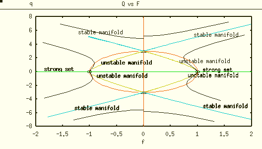
Figure 1: Phase-portrait showing steady states, stable and unstable manifolds of saddle-type steady states, strong sets of stable steady states, and a few other representative orbits with κ = 3 and η = 0.1
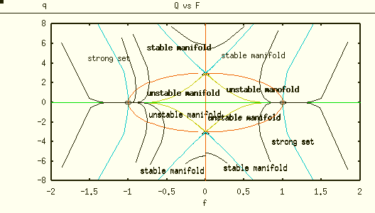
Figure 2: Phase-portrait showing steady states, stable and unstable manifolds of saddle-type steady states, strong sets stable steady states, and a few other representative orbits with κ = 3 and η = 0.01
Remark 1. It is important to point out that actual derivation of the separatrix presents certain difficulties since being on a separatrix is a non-local condition for a point. The future work may address the constructive behavior of separatrix appeared in Figure 1 and Figure 2 in the vicinity of other steady states of the system. In addition, one might be interested in constructing Lyapunov functional to prove the global stability of PLE.
Next, we present the numerical behaviors of solutions \((f, q)\) of the system (3) in Figure 3 for different values of \(\eta\) and various initial conditions. Here \(\kappa\) is chosen to be 3.
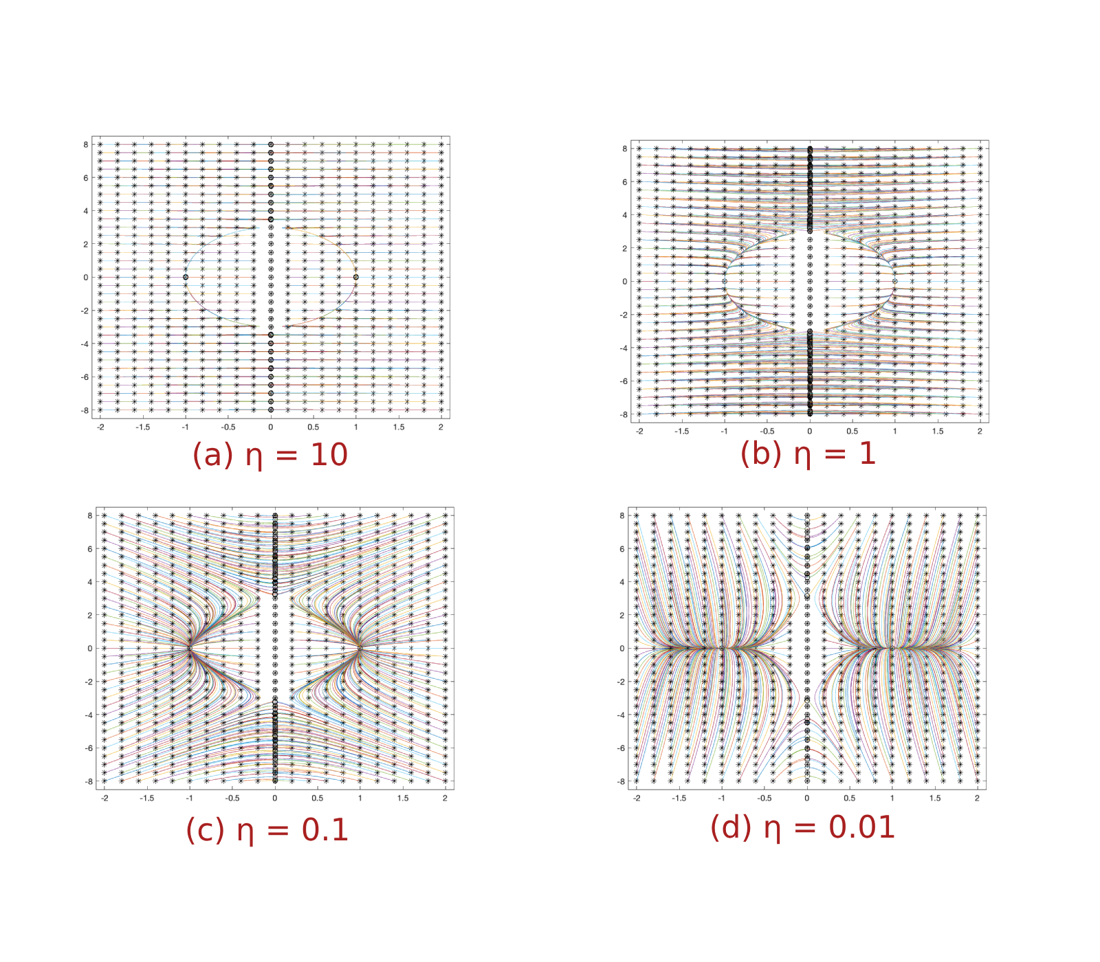
Figure 3: Solutions (f, q) of the unforced system with κ = 3
We observe that solutions of the unforced system converge either to the equilibrium points \((1, 0)\) or \((0, q)\) with \(q > \kappa ( = 3)\). Moreover, there are two regions in the plane, denoted by \(R_{(0, q)}\) and \(R_{(1,0)}\). When initial values \((f_0, q_0)\) are in the region \(R_{(0,q)}\), solutions converges to the equilibrium points \((0, q)\), while when initial values are in the region \(R_{(1,0)}\), solutions converge to the equilibrium point \((1, 0)\). These two regions are roughly divided by a curve/line which depends on values of \(\kappa\) and \(\eta\). The curve/line intersects the \(q-\)axis at \((0, \kappa)\) and as \(\eta\) becomes smaller, the curve/line becomes steeper.
Similar phenomenon can also be observed for \(\kappa = 4\) in Figure 4.
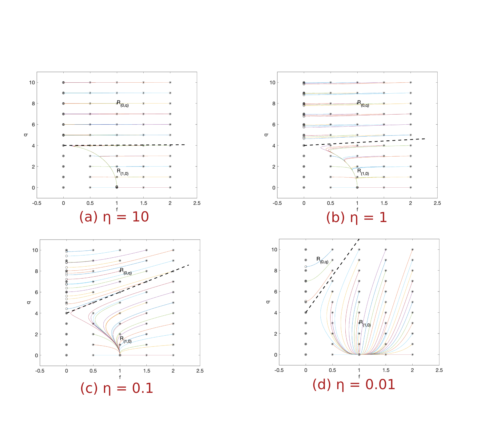
Figure 4: Solutions (f, q) of the unforced system with κ = 4
These results indicate that if the initial magnetic potential of the conductor is sufficiently high, its superconductivity will eventually disappear. On the contrary, the conductor will possess superconductivity and its internal magnetic potential will disappear.
To support this observation, we present how \(f\) and \(q\) change as time elapse for \(\kappa = 3\) and \(\eta = 1\) with two different initial values \((f_0, q_0) = (2, 2) \in R_{(1, 0)}\) and \((f_0, q_0) = (2, 8) \in R_{(0, q)}\) in Figure 5.
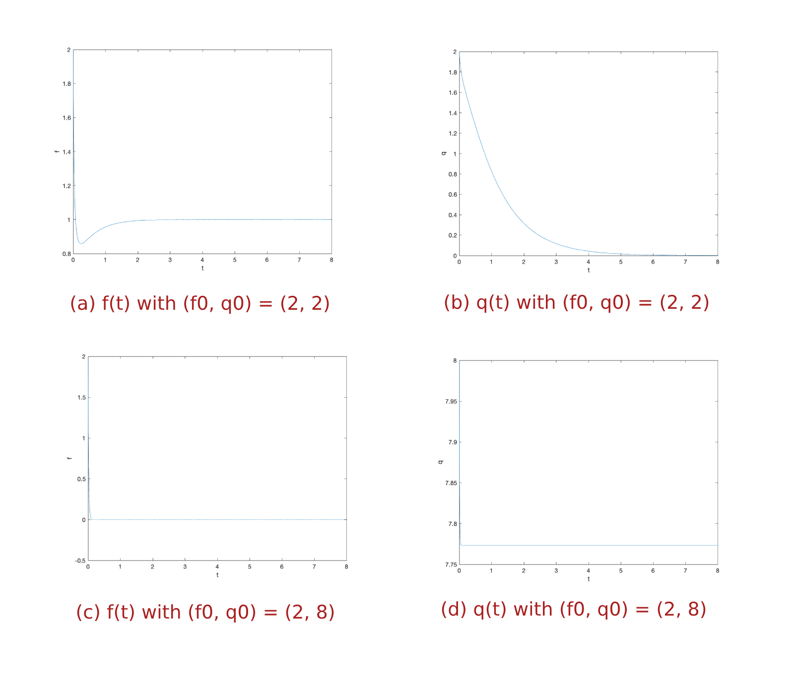
Figure 5: Dynamical behaviors of f(t) and q(t) with κ = 3 and η = 1
Forced Case
One of the significant features of phase lock equation appeared in superconductivity is its attracting set and basin of attraction. As presented so far in Section 2, the speed of attraction is resident in the system’s behavior without the inclusion of the outside forcing function. It is at this point in our exploration of the phase lock equation where we numerically and graphically explore the phase lock with a variety of forcing functions and parameter values.
Let \[h = \alpha \sin (\omega t) + \alpha + \epsilon\] where \(\epsilon\) is a small positive number to guarantee \(h > 0\). Then we have \(0 < \epsilon \leq h \leq 2 \alpha + \epsilon\).
Following Theorem 1, we know that in order to guarantee the existence of periodic solutions, values of \(c, W\) and \(\kappa\) should satisfy \[0 < c \leq \sqrt{1 - \frac{W^2}{\kappa}} < 1 \quad \hbox{and} \quad c W - h \geq 0,\] where \(c\) is a positive constant.
Since \(h \leq 2 \alpha + \epsilon\), to satisfy \(c W - h \geq 0\), we can choose \(W = \displaystyle\frac{2 \alpha + \epsilon}{c}\).
Moreover, \(\displaystyle\sqrt{1 - \frac{W^2}{\kappa}} < 1\), implies \(\kappa > 0\), and from \(\displaystyle c \leq \sqrt{1 - \frac{W^2}{\kappa}}\), we obtain \(\displaystyle c^2 \leq 1 - \frac{(2 \alpha + \epsilon)^2}{c^2 \kappa}\), which leads to \[\label{eq:forcedkappa} \kappa \geq \frac{(2 \alpha + \epsilon)^2}{c^2 (1 - c^2)}.\]
For numerical experiments that we present in this section, without loss of generality, we select \(\omega = 2 \pi, \epsilon = 0.0001\), and \(c = 0.7\).
We first choose the value of \(\alpha\) to be 1. Then by the inequality (4), we define \(\kappa = 16.0080\). Solutions of the forced system (2) are presented in Figure 6.
Compared with the results in the case \(h = 0\), some similar behaviors can be observed. For example, The plane is divided into two regions by a curve/line starting around \((0, \kappa)\). Also, as the value of \(\eta\) becomes smaller, the curve/line is steeper.
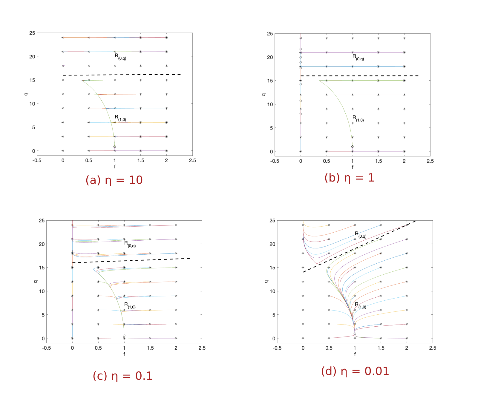
Figure 6: Solutions (f, q) of the forced system with h = sin(2πt) + 1.0001
However, as we look into the dynamical behaviors \(f(t)\) and \(q(t)\) for more details, differences between forced and unforced cases can be observed. To observe these differences, we perform similar simulations of \(f(t)\) and \(q(t)\) for \(\eta = 1\) as we did in Figure 5. Here the two initial conditions that we select are \((f_0, q_0) = (2, 2) \in R_{(1, 0)}\) and \((f_0, q_0) = (2, 20) \in R_{(0, q)}\) (ref. Figure 7.
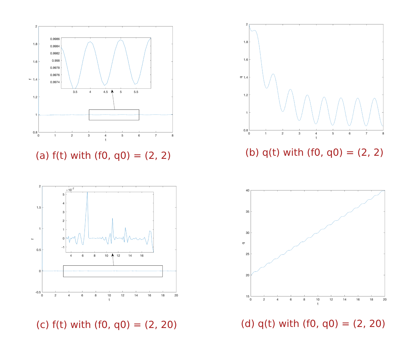
Figure 7: Dynamical behaviors of f(t) and q(t) with h = sin(2πt)+1.0001 and η = 1
First of all, because of the oscillating property of the external forcing function \(h\), solutions here show oscillating behavior. In addition, when initial values are in the region \(R_{(1,0)}\), unlike the unforced case in which solutions converge to the point \((1, 0)\), solutions of the forced system eventually oscillate around \((1, \alpha)\). When initial conditions are in the region \(R_{(0,q)}\), instead of converging to the point \((0, q)\) with \(q > \kappa\), solutions oscillate around 0 in the \(f-\)direction and oscillating increase without bound in the \(q-\)direction.
To observe how the value of \(\alpha\) affects the behaviors of solutions, in Figure 8, we change the value of \(\alpha\) to 3, and present solutions of system (2) with \(h = 3 \sin (2 \pi t) + 3.0001\), in which we choose \(\kappa = 144.0624\) by using (4)
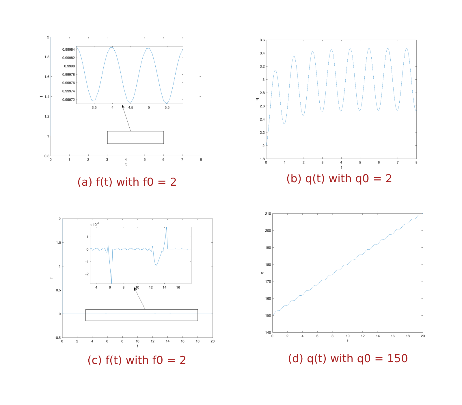
Figure 8: Dynamical behaviors of f(t) and q(t) with h = 3 sin(2πt) + 1.0001 and η = 1
Similar behaviors can be observed. However, in this case, \(q(t)\) oscillates around 3 instead around 1 when \(q_0\) is small.
Explore Unforced and Forced System with Negative Diffusivity
In this section, we discuss solutions of system (2) with negative diffusivity \(\eta\).
We first show numerical results of the unforced case, that is \(h = 0\), in Figure 9 with different negative values of \(\eta\). As the same as what we analyzed in Section 2, for \(\eta < 0\), if initial internal potential of the conductor is positive, then the equilibrium \((1, 0)\) is unstable and the conductivity of the conductor will decrease to zero eventually.
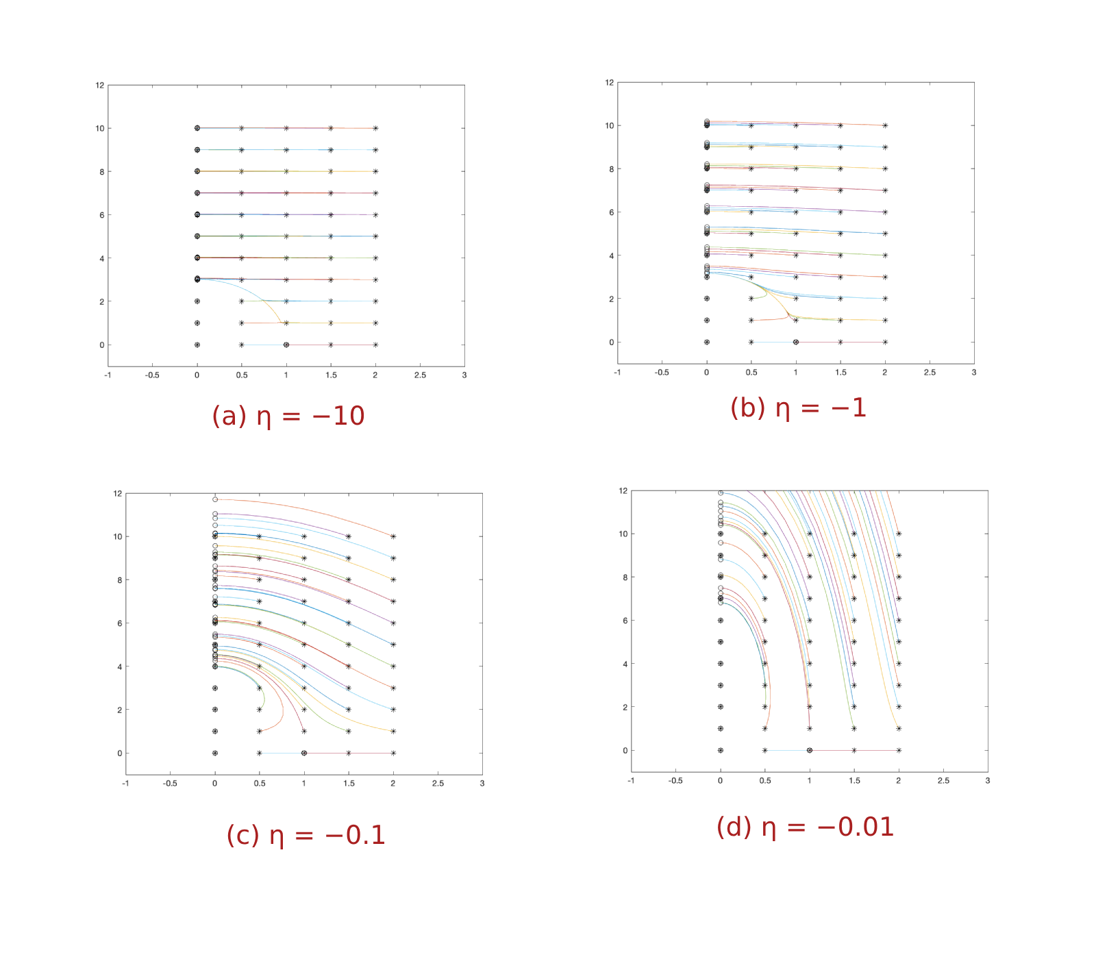
Figure 9: Solutions of the unforced system with κ = 3 and various negative η values
Moreover, to look into the details of the behaviors of \(f(t)\) and \(q(t)\), Figure 10 presents \(f(t)\) and \(q(t)\) for \((f_0, q_0) = (2, 0)\) and \((f_0, q_0) = (2, 2)\) with \(\eta = -1\).
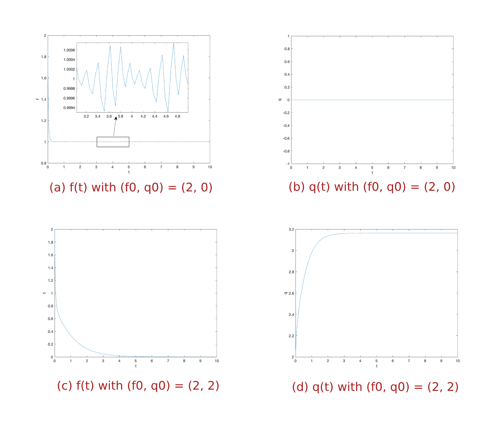
Figure 10: Solutions of the unforced system with κ = 3 and various negative η values
Next, we discuss the system with positive periodic external forces and different negative values of \(\eta\). Let \(h = \sin (2 \pi t) + 1.0001\), the numerical results are shown in Figure 11. Compared with the unforced case, we can observe quite different behaviors of solutions.
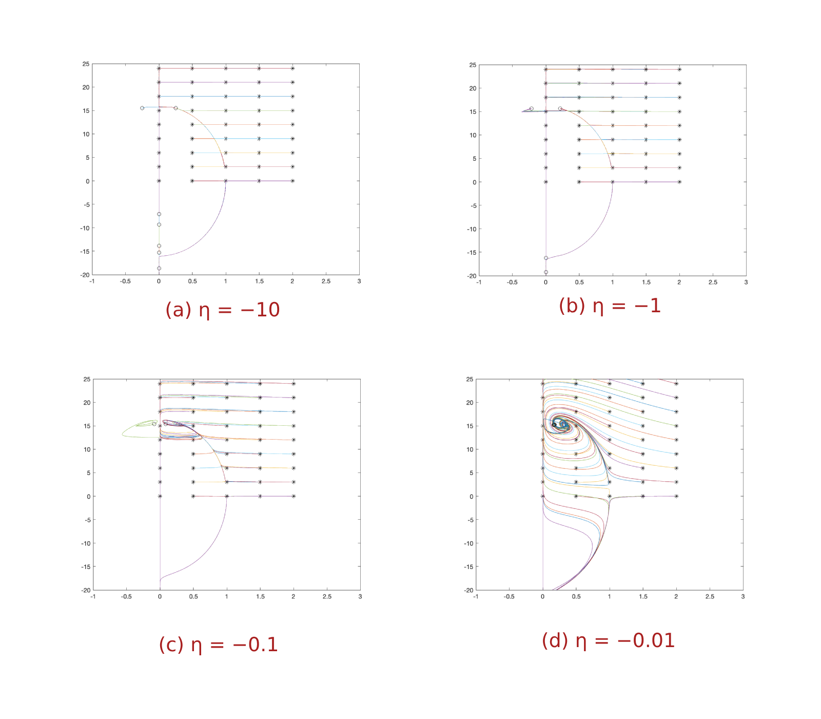
Figure 11: Solutions of the forced system with various negative η values
In addition, numerical behaviors of \(f(t)\) and \(q(t)\) with different initial conditions are presented in Figure 12, in which we use \(\eta = -1\). Compared with the results in Figure 7, we can see that they are quite different from each other, and one is not merely the reverse of another.
Figure 12: f(t) and q(t) for the forced system with h = sin(2πt) + 1.0001 and η = −1
Conclusion Remarks
In conclusion, we investigate the dynamical and qualitative behaviors of phase-lock equations arising in superconductivity, modeled as nonlinear ordinary differential equations. By selecting different values of the Ginzburg-Landau parameter \(\kappa\) and the diffusivity parameter \(\eta\), we identify varying attracting regions for solutions corresponding to various initial conditions. Additionally, the presence of periodic external noise induces oscillatory behaviors in the solutions. Despite these variations, the qualitative behaviors of the solutions remain consistent across all cases. This model system can be further developed to generate domain of attraction in superconductivity in the field of physics and engineering. The authors found that phase-lock model arises in superconductivity to be both challenging and mathematically interesting through the exploration of how different range parameter values influence the system. Hopefully, future research will address global qualitative and quantitative behavior and new applications of this model system.
Acknowledgment
The authors would like to thank the referees for the valuable suggestions that contributed to a significant improvement of the paper.
Conflict of Interest
There is no conflict of interest.
References
Beasley, M. R. (2009). Notes on the Ginzburg-Landau Theory, ICMR Summer School on Novel Superconductors University of California, Santa Barbara. View
Fan, J., Nakamura, G., and Zhan M. (2021). Uniqueness and Decay of Weak Solutions to Phase-Lock Equations. Discontinuity, Nonlinearity, and Complexity, 10(1), 31-41. View
Konsin, P. and Sorkin, B. (2009). Time-dependent Ginzburg-Landau equations for a two-component superconductor and the doping dependence of the relaxation times of the order parameters in Y Ba2Cu3O7−δ, Journal of Physics: Conference Series 150, View
Wang, B. (1999). Existence of Time Periodic Solutions for the Ginzburg-Landau equations of superconductivity, J. Math. Anal. & Appl. 232, 394-412. View
Wang, S. and Zhan, M. (1999) L p Solutions to Time Dependent Ginzburg-Landau Equations of Superconductivity, J. Non. Anal. 36, 661-677. View
Xie, H., Fan, J., and Zhou, Y. (2020). Global well-posedness of weak and strong solutions to the nD phase-lock system. Applicable Analysis, 101(1), 167–172. View
Zhan, M. (2000). Existence of Periodic Solutions for Ginzburg-Landau Equations of Superconductivity, J. Math. Anal. & Appl. 249, 614-625. View
Zhan, M. (2008). Multiplicity and Stability of Time-periodic Solutions of Ginzburg-Landau Equations of Superconductivity, J. Math. Anal. & Appl. 340, 126–134. View
Zhan, M. (2000). Phase-Lock Equations and its Connections to Ginzburg -Landau Equations of Superconductivity, J. Non. Anal. 42,1063-1075.
Zhan, M. (2005). Well Posedness of Phase-Lock Equations of Superconductivity, J. Appl. Math. Letters 8, 1210-1215. View